
Friction forces#
So far we have assumed ideal, frictionless joints. Real machines have passive resistances that oppose relative motion, dissipate energy (heat, wear) and reduce efficiency: part of the input work is lost as passive work instead of becoming useful work (see efficiency in lesson 4). In other cases, friction is precisely what makes the mechanism work: brakes, clutches, belts, bar clamps…
Reaction forces and friction forces#
Each joint between two links defines, in each of its relative degrees of freedom, one of these two kinds of forces:
Reaction forces: they are as large as needed to prevent relative motion. They are always unknowns to be solved.
Friction (passive) forces: they oppose relative motion, without totally preventing it. They always have known expressions (the friction models on this page).
If friction is large enough to totally block the relative motion, the friction force “becomes” a reaction. In each degree of freedom only one of the two can exist.
Kinds of relative motion at a contact#
There are friction forces (or moments) for each of the three kinds of relative motion between two bodies in contact at a point \(J\):
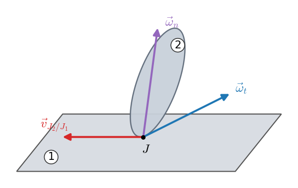
Sliding: the contact points of both bodies (\(J_1\) and \(J_2\)) have a relative translational velocity, within the common tangent plane: \(\vec{v}_{J_2/J_1} \neq \vec{0}\).
Rolling: relative rotation about an axis tangent to the surfaces at \(J\) (component \(\vec{\omega}_t\) of the relative angular velocity).
Pivoting: relative rotation about an axis perpendicular to the surfaces at \(J\) (component \(\vec{\omega}_n\)).
Sliding friction#
Tangential forces between solids in contact have complex origins: roughness, micro-welding, molecular forces… Engineering uses simplified models.
Coulomb’s model (dry friction)#
Between two bodies in contact with dry friction, the friction force \(F_f\) opposes the motion (or the tendency to move) and satisfies:
\(N\): normal force at the contact.
\(\mu\): friction coefficient, dimensionless (typical values between 0.01 and 0.8).
\(\mu_e\): static coefficient, if there is no relative motion. While \(F_f < \mu_e N\), the friction force is a reaction: it is as large as needed to prevent sliding.
\(\mu_d\): kinetic (or dynamic) coefficient, if there is relative motion. Then \(F_f = \mu_d N\), opposite to the relative velocity. It is approximately constant, and \(\mu_d < \mu_e\).
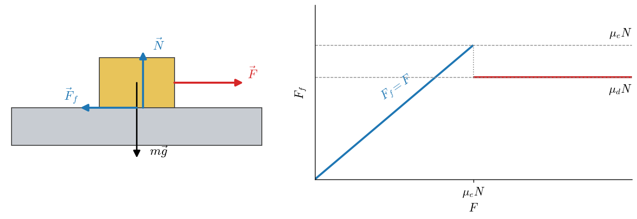
In vector form, while sliding: \(\vec{F}_f = -\mu_d\, N\, \dfrac{\vec{v}_{rel}}{|\vec{v}_{rel}|}\).
The friction coefficient depends on the nature of the surfaces in contact, their condition (roughness, cleanliness, lubrication, temperature), their relative arrangement and the duration of the contact. Some typical values:
Materials |
\(\mu_e\) (dry) |
\(\mu_d\) (dry) |
\(\mu_d\) (lubricated) |
|---|---|---|---|
Steel on steel |
0.74 - 0.80 |
0.42 - 0.62 |
0.03 - 0.19 |
Aluminum on steel |
0.61 |
0.47 |
|
Brass on steel |
0.35 - 0.51 |
0.44 |
|
Copper on steel |
0.53 |
0.36 |
0.18 |
PTFE (Teflon) on steel |
0.04 - 0.2 |
0.04 |
0.04 |
Wood on metal |
0.2 - 0.6 |
0.49 |
0.075 |
Rubber on concrete |
1.0 |
0.6 - 0.85 |
0.45 - 0.75 (wet) |
Ice on ice |
0.02 - 0.09 |
(Source: Wikipedia, Friction, CC BY-SA.) In machine design, reference values such as \(\mu = 0.12\) (\(\varphi \approx 7^\circ\)) are used for slides, cams, eccentrics and gears; \(\mu = 0.10\) (\(\varphi \approx 6^\circ\)) for revolute joints; \(\mu = 0.20\) (\(\varphi \approx 12^\circ\)) for unlubricated joints, and \(\mu = 0.30\) (\(\varphi \approx 17^\circ\)) for brakes.
Dissipated power#
If a body slides at velocity \(v\) with Coulomb friction, the work of the friction force along a displacement \(ds\) is \(dW = \mu N\, ds\), and the dissipated power (losses through heat and wear) is:
Viscous friction and complete model#
Coulomb’s model does not describe well the contact between surfaces separated by a lubricant. In that case, the viscous friction model is used, proportional to the relative velocity:
with \(c\) the viscous damping coefficient (N·s/m). More complete models combine both effects and the transition between static friction and full lubrication (the Stribeck curve): when sliding starts, the force drops from the static value (boundary and mixed lubrication regimes) and then grows with velocity (full, viscous lubrication).
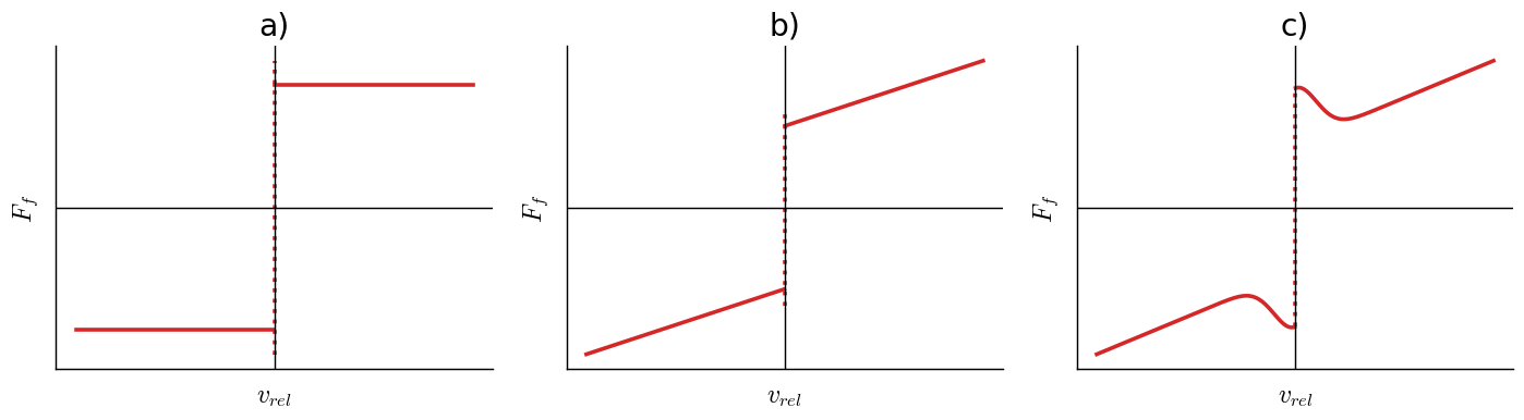
Models: a) Coulomb; b) Coulomb plus viscous; c) with Stribeck effect.
Strategy for solving problems with friction#
The main difficulty is that, a priori, we do not know whether friction will be enough to prevent motion: each joint with friction may be a reaction (locked) or a moving joint with friction forces. Moreover, each combination gives a different kinematic chain, with a different number of degrees of freedom.
Solve the problem assuming there is no sliding, that is, as if all joints with friction were reactions.
Check whether the resulting reactions are larger than allowed by the friction model (\(F_f \le \mu_e N\)).
At the joints where the reactions turn out too large, replace them with moving joints with known friction forces (\(F_f = \mu_d N\), opposite to the motion) and solve again.
In start of motion (or locking) problems, the limit case is written directly: \(F_f = \mu N\) at all the contacts that would slide, with the sense opposite to the motion under study. This is how Example 3.8: Bar clamp (friction locking) and Example 3.9: Two blocks joined by a bar, with friction are solved.
Friction cone#
Adding up the normal and friction forces at a point contact gives the total reaction \(\vec{R}\). Since \(F_f \le \mu N\), the angle between \(\vec{R}\) and the normal cannot exceed the friction angle \(\varphi\):
At a point contact with dry friction, the reaction that can exist (fully preventing motion) has a direction within a cone of half-angle \(\varphi = \arctan\mu\) around the normal, called the friction cone.
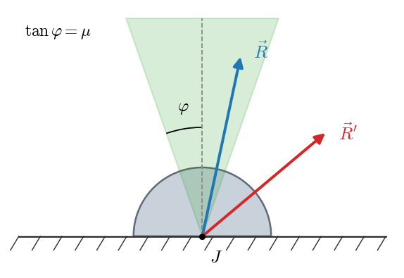
If the resultant of the external forces that one body exerts on the other falls inside the cone (\(\vec{R}\)), the contact balances it and there is no sliding, however large it is. If it falls outside (\(\vec{R}'\)), sliding occurs. With two contacts, the condition applies to each of them: for instance, for a ladder leaning on a wall not to slide, the vertical through the center of gravity of the ladder + person must pass through the region common to the two friction cones at the supports.
A well-known case is the inclined plane: a block at rest on a ramp of angle \(\theta\) starts sliding when \(\theta > \varphi\), that is, when \(\tan\theta > \mu_e\). It is a simple way to measure the static friction coefficient.
In the construction below, a block is pushed with an inclined force \(\vec{P}\); change the angle \(\beta\) and see when the required reaction leaves the cone:
Friction locking (self-locking)#
In general, as the applied force grows, the friction reaction reaches its limit and the body slides. But in some cases the external forces themselves make the normal force \(N\) grow in the same proportion, so the reaction never leaves the cone and motion never happens: the mechanism is self-locking. This effect is the basis of many mechanisms:
The carpenter’s bar clamp: the moving arm tilts and locks on the bar when tightened (Example 3.8: Bar clamp (friction locking)).
The worm drive: if the lead angle is smaller than the friction angle, the worm gear cannot drive the worm.
Wedges, jack screws and ratchets.
Drift#
If two bodies already slide in one direction, the kinetic friction force opposes the total relative velocity. To move the body in another direction (perpendicular, at velocity \(v_d\)), only the friction component along that direction must be overcome, which is a small part of the kinetic friction (itself smaller than the static one):
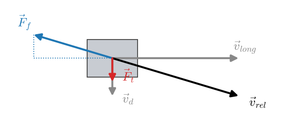
The friction in the drift direction can be made as small as desired by increasing the sliding velocity \(v_{long}\). Applications:
Pulling a cork out of a bottle is easier while twisting it.
In a centrifugal governor, the sleeve rotates on a moving support so that its vertical motion, produced by the change in the centrifugal force of the balls, does not have to overcome static friction.
A skidding vehicle (locked wheels sliding forward) loses its ability to withstand lateral forces and cannot turn: this is the reason for anti-lock braking systems (ABS).
Rolling resistance#
If the contact between a wheel and the ground were really a point, there would be no moment resisting rolling. In reality, the bodies deform elastically and a small contact patch forms, with an asymmetric pressure distribution (higher at the front). The resultant \(\vec{N}\) is shifted forward a distance \(\rho\) and produces a rolling resistance moment, which opposes the relative angular velocity:
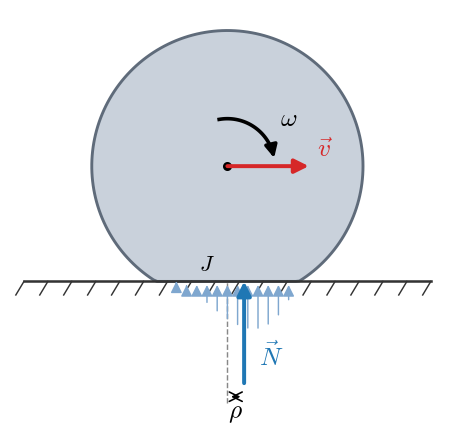
The rolling resistance coefficient \(\rho\) has units of length: it is the distance the resultant of the pressures is shifted. Typical values: wood, \(\rho \approx 0.8\) mm; hardened steel, \(\rho \approx 0.01\) mm. It depends on the rolling speed, the elastic properties of the materials, temperature, contact pressure and radii of curvature.
Rolling or sliding. If a wheel of radius \(r\) is pulled with a horizontal force \(F\) at its center, the wheel:
Rolls when \(F\, r > \rho N\), that is, \(F > \frac{\rho}{r} N\).
Slides when \(F > \mu N\).
Since normally \(\rho/r \ll \mu\), the wheel rolls long before it slides: this is why it is much easier to move a load on wheels than to drag it. See Example 3.10: Sliding door (rolling and sliding).
Pivoting resistance#
Similarly to rolling, pivoting (rotation about the contact normal) produces a pivoting resistance moment, due to sliding friction over the whole contact patch:
Integrating friction over the contact patch (\(dM_p = r\,\mu\,dN\)), with the pressure distribution from Hertz’s theory of contact between elastic bodies, the coefficient \(\rho_p\) is proportional to \(\mu\) and to the size of the contact patch, which depends on the load and the materials.
Friction at the joints#
Friction at pin joints (revolute joints) is modeled with the friction circle: the reaction no longer goes through the center of the pin, but is tangent to a circle of radius \(r_f \approx \mu\, r\) (with \(r\) the radius of the pin), so that it produces a friction torque opposing the relative rotation. This model, friction at prismatic guides and machine efficiency are studied in lesson 4 (Lesson 4: Basic Concepts of Work and Energy Applied to Mechanisms).
Friction-based mechanisms#
Although friction is undesirable in most machines, many mechanisms work thanks to it:
Motion transmission: friction wheels, belts, feed rollers, rolling mills.
Clutches and brakes (for instance, the Prony brake, used to measure engine torque).
Locking mechanisms: wedge presses, bar clamps, self-locking screws.
Examples#
Example 3.8: Bar clamp (friction locking): maximum width of the arm of a bar clamp so that it does not slide.
Example 3.9: Two blocks joined by a bar, with friction: force to start the motion of two blocks joined by a bar, with dry friction.
Example 3.10: Sliding door (rolling and sliding): sliding door with rollers that roll or slide.