Particle dynamics

Before moving on to rigid bodies, we review the basic concepts of the dynamics of a particle (a point with mass \(m\) and no dimensions).

Linear momentum

Definition

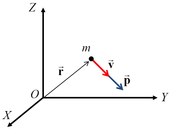
The linear momentum of a particle is the vector quantity, given in an inertial reference frame:

\[\vec{p} = m \vec{v}\]

Newton’s second law

\[ \vec{F} = \dot{\vec{p}} \]

Principle of conservation of linear momentum

\[ \vec{F} = \vec{0} \quad \rightarrow \quad \vec{p} = \text{constant} \]

Angular momentum

Definition

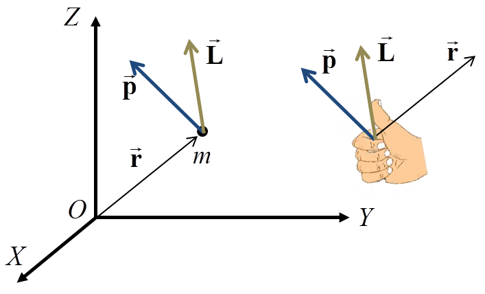
The angular momentum of a particle about a point \(O\) is:

\[ \vec{L}_O = \vec{r} \times \vec{p} \]

where \(\vec{r}\) is the position vector of the particle from \(O\).

Cross-multiplying Newton’s second law by \(\vec{r}\):

\[ \underbrace{\vec{r} \times \vec{F}}_{\vec{M}_O} = \vec{r} \times \dot{\vec{p}} \]

On the other hand, differentiating the angular momentum with respect to time (with \(O\) fixed):

\[ \frac{d\vec{L}_O}{dt} = \frac{d}{dt}\left( \vec{r} \times m\vec{v} \right) = \underbrace{\vec{v} \times m\vec{v}}_{=\vec{0}} + \vec{r} \times \dot{\vec{p}} = \vec{r} \times \dot{\vec{p}} \]

since the cross product of a vector with itself is zero. Comparing both expressions:

Rate of change of the angular momentum

\[ \vec{M}_O = \vec{r} \times \dot{\vec{p}} = \dot{\vec{L}}_O \]

Principle of conservation of angular momentum

\[ \vec{M}_O = \vec{0} \quad \rightarrow \quad \vec{L}_O = \text{constant} \]

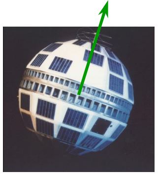
A classic application of this principle is spin stabilization of satellites: Telstar I (1962) spun about its major axis at about 200 rpm to keep its orientation.

Equations of motion of a particle

For a particle we have the system of differential equations:

\[\begin{split} \begin{aligned} \vec{F} &= \dot{\vec{p}} &\qquad& \text{(Newton, 1643-1727)} \\ \vec{M}_O &= \dot{\vec{L}}_O &\qquad& \text{(Euler, 1707-1783)} \end{aligned} \end{split}\]

In 3D these are six scalar equations, but for a point particle they are redundant: the second one follows from the first, as we have just seen. Newton’s equation is therefore enough. Since \(\dot{\vec{p}} = \frac{d}{dt}(m\vec{v}) = \frac{d}{dt}(m\dot{\vec{r}}) = m\ddot{\vec{r}}\) (with constant \(m\)):

\[ m \ddot{\vec{r}} = \vec{F} \]

which is a system of three ordinary differential equations (ODE):

\[\begin{split} \begin{aligned} \ddot{x}(t) &= \frac{1}{m} F_x(t) \\ \ddot{y}(t) &= \frac{1}{m} F_y(t) \\ \ddot{z}(t) &= \frac{1}{m} F_z(t) \end{aligned} \end{split}\]

This system can be solved analytically in simple cases or, in general, with numerical integrators (Euler’s rule, trapezoidal rule, Runge-Kutta…).

Example: numerical integration with Euler’s rule

To integrate \(m\ddot{x} = F(t, x, \dot{x})\), it is written as a first-order system with state \((x, v)\) and advanced with a time step \(\Delta t\):

\[\begin{split} \begin{aligned} v_{k+1} &= v_k + \frac{\Delta t}{m} F(t_k, x_k, v_k) \\ x_{k+1} &= x_k + \Delta t\, v_k \end{aligned} \end{split}\]

For instance, for a mass on a spring (\(F=-kx\)), in MATLAB:

m = 1; k = 10; dt = 1e-3; N = 5000;
x = zeros(1,N); v = zeros(1,N); x(1) = 0.1;
for i = 1:N-1
    v(i+1) = v(i) + dt/m * (-k*x(i));
    x(i+1) = x(i) + dt * v(i);
end
plot((0:N-1)*dt, x)

Euler’s rule is the simplest but accumulates error (in this example the amplitude slowly grows); in practice, higher-order methods such as ode45 are used.