Robot Forward Kinematics Simulator#
Introduction#
Robot kinematic analysis consists of studying the relationship between the value assigned to the degrees of freedom (joint coordinates) and the position and orientation (pose) of the end effector, as well as its position and acceleration. This analysis can respond to the resolution of the direct or inverse kinematic problem, depending on whether the input data is referred to the joint space or the end effector space (task space).
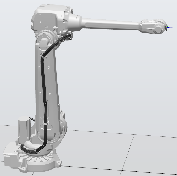
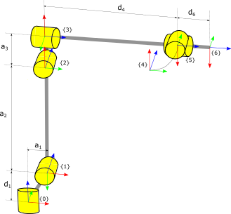
In this simulator the forward kinematic problem is implemented. To do this, the kinematic chain of the robot under study is first defined, based on the standard Denavit–Hartenberg parameters. To exemplify this procedure a CAD model of the ABB IRB 4600 robot is shown in the Figure (left), while its schematic according to this convention is shown at the rigth. The resulting parameters are summarized in the Table.
Once the DH parameter table is available, it must be saved in a .txt file like the one you can download at this link. These corresponds to the ABB IRB 4600, wich are the followings:
\(a_i\) |
\(\alpha_i\) |
\(d_i\) |
\(\theta_i\) |
Jt |
|---|---|---|---|---|
0.175 |
-90 |
0.495 |
0 |
1 |
1.095 |
0 |
0 |
-90 |
1 |
0.175 |
-90 |
0 |
0 |
1 |
0 |
90 |
1.2305 |
0 |
1 |
0 |
90 |
0 |
180 |
1 |
0 |
0 |
0.085 |
0 |
1 |
where Jt is the joint type, being 1 for revolute joints and 2 for prismatic joint. Then, the simulator can be run and that table loaded. A 3D view of the analyzed robot will automatically be generated, and the pose data in the initial position is displayed. To define a new pose, the sliders corresponding to each of the joints that the robot has will be used. In this case, there are 6 joints, all of them being revolution. You can see how the data of the new pose is updated as the robot moves, while a trace is generated with the trajectory that the end effector describes.
The Simulator#
The following iframe corresponds to the RobotFKS simulator. To start a session, click on Run and then load the .txt file with the DH parameter table. Then, use the sliders to define new configurations.
Other types of robots#
When dealing with prismatic joints, it is necessary to include a fifth column in the DH parameter table defining the joint type. Thus, a value of 2 must be set for prismatic joints, and 1 for those of revolution. In the following links you can download the configuration files corresponding to various types of robots with different types and numbers of joints:
RPR concept robot DH table
KUKA LBR iiwa (7 DOF) DH table
Schunk LWA 4P DH table
PRR concept robot DH table
PPP concept robot DH table
Example of use:
Conclusions#
The RobotFKS tool constitutes a light and effective tool for solving the direct kinematic problem of robots composed of open kinematic chains and revolution and prismatic joints. Its minimalist interface and the fact that it can be run directly from a web browser [1], without having to install any program, make it a very useful complement in robotics learning. Specifically, it can be of great help in the initial modeling stage, to verify the correct assimilation of the concepts related to the implementation of the Denavit–Hartenberg method, and later, in the calculation of direct kinematics. These two tasks are crucial in both programming and design of robots. As future work, the improvement of the rendering of the links can be considered, when there are prismatic type joints followed by a non-zero value of the parameter ‘a’ as well as the end effector.