Lesson 5: Fundamentals of Machine Balancing#
1. Introduction: Why do we balance?#
In machine design, any rotating element (rotor) has a mass distribution that is never theoretically perfect. Manufacturing tolerances, non-homogeneous materials, or wear cause the center of gravity to be misaligned with respect to the rotation axis.
This non-homogeneity translates into eccentric masses (masses \(m\) located at a radius \(\vec{r}\) from the rotation axis). When the rotor spins at an angular velocity \(\vec{\omega}\), these masses generate centrifugal inertia forces.
Since the rotor is rotating, these forces also rotate, transmitting cyclic loads to the bearings and to the ground. This causes:
Vibrations: The main cause of noise and fatigue failures in the machine and its mounts.
Accelerated wear: Destruction of bearings and bushings.
Loss of quality: In machine tools (grinders, lathes), vibrations prevent an accurate finish.
Balancing is the process of adding (or removing) correction masses so that the resultant of all the inertia forces and moments becomes zero, allowing the rotor to spin without vibrating. This video shows an example of this phenomenon. Likewise, this other video shows how the balancing process can be carried out with an industrial machine.
2. The Physical Origin: Axes and Forces#
Unbalance is a misalignment between two axes:
Rotation Axis: The geometric line defined by the centers of the bearings.
Principal Axis of Inertia (PAI): The natural axis of the body’s mass distribution.
A rotor is perfectly balanced only if its Principal Axis of Inertia coincides with its Rotation Axis. Any misalignment causes vibration problems.
Reminder: What is the Principal Axis of Inertia (PAI)?#
The Principal Axis of Inertia (PAI) is a mass-symmetry axis. If a body spins freely in space (without bearings, like an asteroid), it will always rotate stably about one of its three PAIs.
Why does it matter? When we force a rotor to spin about an axis (the bearing axis) that is not its PAI, the rotor “fights” to rotate about its PAI instead.
The effect: This “fight” is what generates tipping forces and moments that try to realign the rotor, causing vibrations. The goal of dynamic balancing is, in essence, to modify the rotor’s mass distribution (by adding masses) so that its PAI aligns with the rotation axis.
3. Types of Unbalance#
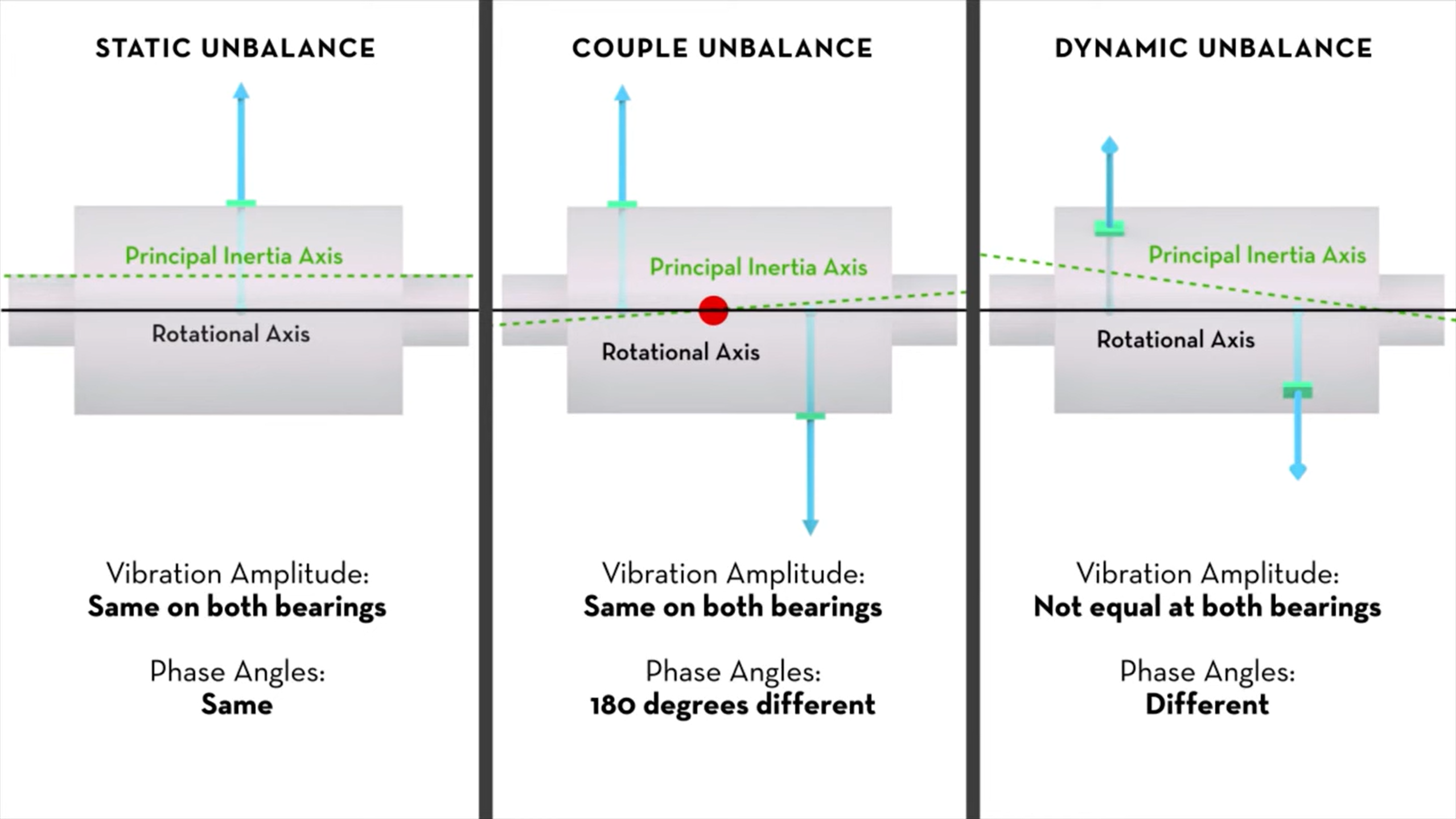
Depending on the geometric relationship between the Principal Axis of Inertia (Inertia Axis) and the Rotation Axis, we distinguish three fundamental cases. This video illustrates the concepts excellently.
3.1 Static Unbalance#
Geometry: The Inertia Axis is parallel to the Rotation Axis, but offset from it.
Physical effect: The center of gravity (G) is not on the axis. A net centrifugal force (shaking force) is generated, but there is no tipping moment if measured about the center of gravity.
Detection: Detected statically (by gravity, using knife edges). The two bearing reactions have the same direction and phase.
Solution: Corrected in a single plane.
3.2 Couple Unbalance#
Geometry: The Inertia Axis crosses the Rotation Axis at the center of gravity (G), but is tilted with respect to it.
Physical effect: The center of gravity (G) is exactly on the rotation axis (so the sum of forces is zero), but the mass is distributed asymmetrically on either side. This creates a pure couple (tipping couple) that tries to rotate the axis.
Detection: Not detectable statically (the rotor would stay still on knife edges). It is only noticeable while spinning. The bearing reactions are equal but opposite (180° out of phase).
Solution: Requires two correction planes.
(Note: it is called a “couple” unbalance because it comes from the mechanical concept of a “couple” — a pure moment with no resultant force.)
3.3 Dynamic Unbalance#
Geometry: This is the most general and common case. The Inertia Axis neither coincides with nor crosses the Rotation Axis (they are skew in space).
Physical effect: It is a combination of the two previous cases. There is both a shaking force (offset G) and a tipping couple (tilted axis).
Detection: Requires dynamic measurement. The bearing reactions have different amplitudes and phases.
Solution: Requires two correction planes.
4. Mathematical Formulation and Simplification#
4.1 Centrifugal Force (Vector vs. Scalar)#
The (vector) inertia force generated by a mass \(m_i\) rotating at a vector angular velocity \(\vec{\omega}\) with radius vector \(\vec{r}_i\) is:
\(\vec{F}_i = m_i \cdot \vec{a}_n = m_i \cdot (\vec{\omega} \times (\vec{\omega} \times \vec{r}_i))\)
For our usual calculations (with \(\vec{\omega}\) aligned with the Z axis and \(\vec{r}_i\) in the XY plane), this force is radial and its magnitude (scalar) is computed as:
\(F_i = m_i \cdot r_i \cdot \omega^2\)
(Note: in this last expression, \(F_i\), \(r_i\) and \(\omega\) are scalar quantities.)
4.2 The “Unbalance Vector” Simplification#
Since the goal is for the sum of the (vector) forces to be zero (\(\sum \vec{F}_i = \vec{0}\)), and every term contains the scalar \(\omega^2\) (assuming \(\omega\) constant):
\(\sum (m_i \cdot (\vec{\omega} \times (\vec{\omega} \times \vec{r}_i))) = \vec{0}\)
If the rotation is planar (\(\vec{\omega} \perp \vec{r}_i\)), the expression simplifies. We can factor out the scalar \(\omega^2\) from the sum of vectors \(m_i \vec{r}_i\):
\(\omega^2 \sum (m_i \vec{r}_i) = \vec{0}\)
We can simplify by dividing the whole equation by \(\omega^2\). This lets us work with a vector quantity called the Unbalance Vector (\(\vec{U}\)):
\(\vec{U}_i = m_i \cdot \vec{r}_i\)
The force-balance equation reduces to: \(\sum \vec{U}_i = \sum (m_i \cdot \vec{r}_i) = \vec{0}\)
Practical note: In balancing problems we work directly with the unbalance vectors \(m\vec{r}\) (units kg·m). This is what the MATLAB code in Example 5.01 computes. If the system is balanced for \(m\vec{r}\), it is balanced for any speed \(\omega\) (for rigid rotors).
5. Single-Plane Balancing (Static Case)#
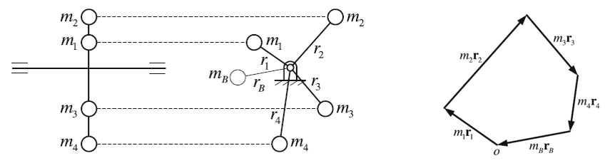
Used for “narrow” rotors (flywheels, pulleys, discs) where all the unbalance is assumed to be concentrated in a single plane perpendicular to the axis. It only corrects the shaking force (Static Unbalance).
The equation is a simple vector sum of unbalances: \(\sum \vec{U}_i = \vec{0} \quad \Rightarrow \quad (m_1 \vec{r}_1 + m_2 \vec{r}_2 + \dots) + m_c \vec{r}_c = \vec{0}\)
Where \(m_c \vec{r}_c\) is the unbalance vector of the correction mass we need to add to close the force polygon.
6. Two-Plane Balancing (Dynamic Case)#
This is the general method for any elongated rigid rotor. It is needed to correct both Couple Unbalance and Dynamic Unbalance. To cancel out both effects (force and moment), correction masses are needed in two different planes (\(A\) and \(B\)).
Two conditions must be satisfied simultaneously:
Force balance (vectors \(\vec{U} = m\vec{r}\)): Prevents the center of gravity from moving. \(\sum \vec{U}_i = \vec{0} \quad \Rightarrow \quad \sum_{i=1}^{n} (m_i \vec{r}_i) + m_A \vec{r}_A + m_B \vec{r}_B = \vec{0}\)
Moment balance (vectors \(\vec{M}\)): Prevents the axis from pitching. The moment of each unbalance vector about an origin \(O\) is \(\vec{M}_i = \vec{d}_i \times \vec{U}_i\), where \(\vec{d}_i\) is the axial position vector. \(\sum \vec{M}_i = \vec{0} \quad \Rightarrow \quad \sum_{i=1}^{n} (\vec{d}_i \times m_i \vec{r}_i) + (\vec{d}_A \times m_A \vec{r}_A) + (\vec{d}_B \times m_B \vec{r}_B) = \vec{0}\)
7. Analytical Solution Method#
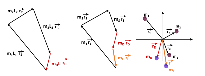
The vector system of equations above is solved systematically (exactly as the MATLAB script does) following these steps:
Pick a smart origin: Take the position of one of the unknown correction planes, e.g. Plane A, as the moment origin (\(d=0\)).
Simplify moments: By setting \(\vec{d}_A = \vec{0}\), the moment generated by correction mass A becomes zero. One unknown disappears.
Solve for Plane B: The moment equation now has only one vector unknown (\(m_B \vec{r}_B\)), which can be solved directly. \(\sum_{i=1}^{n} (\vec{d}_i \times m_i \vec{r}_i) + (\vec{d}_B \times m_B \vec{r}_B) = \vec{0}\)
Solve for Plane A: Once the correction at B is known, go back to the force equation. Now the only unknown is A, obtained by a simple vector subtraction. \(\sum_{i=1}^{n} (m_i \vec{r}_i) + m_A \vec{r}_A + (m_B \vec{r}_B)_{\text{known}} = \vec{0}\)