Velocity Analysis#
Once the position is known, we can determine the velocities.
Relative Velocity Method (Graphical and Analytical)#
This is the most fundamental method and is based on the relative velocity equation between two points A and B: \( \vec{v}_B = \vec{v}_A + \vec{v}_{B/A} \) The key term is \(\vec{v}_{B/A}\), the velocity of B relative to A. If A and B belong to the same rigid link, there can be no change in the distance between them. The only possible relative motion is rotation. Therefore, the velocity \(\vec{v}_{B/A}\) is the result of the rotation of link AB around A, and its vector is always perpendicular to the segment AB.
This property is the basis of the graphical method of the velocity polygon:
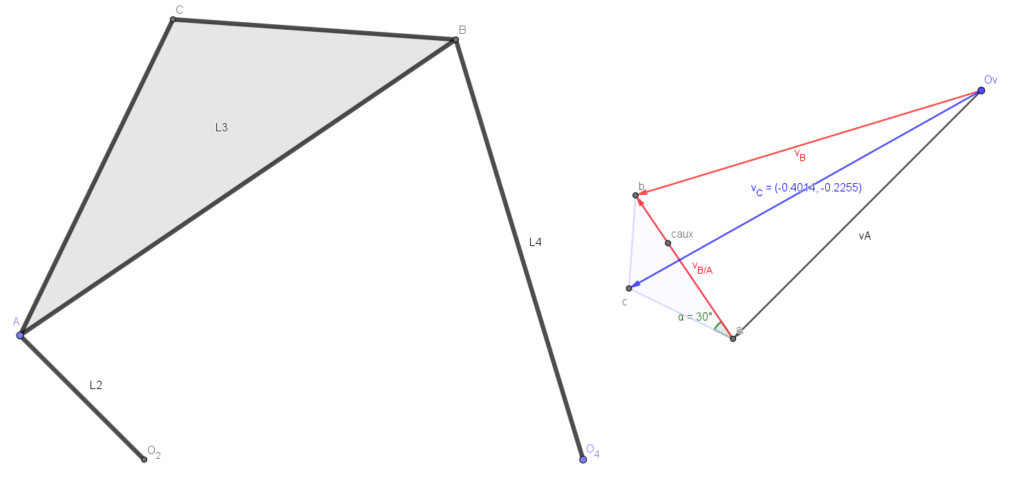
Velocity origin: A point (\(O_v\)) is chosen to represent zero velocity (the frame).
Known vector: The first known velocity vector is calculated and drawn to scale. For example, \(\vec{v}_A = \vec{\omega}_2 \times \vec{R}_A\), which is perpendicular to \(O_2A\). It is drawn from \(O_v\).
Construct the equation: For the equation \(\vec{v}_B = \vec{v}_A + \vec{v}_{B/A}\), we know that:
The direction of \(\vec{v}_B\) is perpendicular to \(O_4B\) (pure rotation around \(O_4\)). A line with this direction is drawn from the origin \(O_v\).
The direction of \(\vec{v}_{B/A}\) is perpendicular to \(AB\). A line with this direction is drawn from the tip of the vector \(\vec{v}_A\).
Close the polygon: The intersection of these two lines defines the tips of the vectors \(\vec{v}_B\) and \(\vec{v}_{B/A}\). By measuring their lengths to scale, we obtain their magnitudes and, from them, the angular velocities \(\omega_3 = |\vec{v}_{B/A}| / L_{AB}\) and \(\omega_4 = |\vec{v}_B| / L_{O4B}\).
Homology and Velocity of any Point#
The velocity polygon is a scale image of the mechanism, rotated 90°. This property, known as homology, is extremely useful. To find the velocity of any point C on the coupler AB, it is sufficient to locate a point c on the segment ab of the velocity polygon, such that the ratio of distances is maintained: \(AC/AB = ac/ab\). The vector from \(O_v\) to c will be the velocity vector \(\vec{v}_C\).
Instantaneous Centers of Rotation (ICR) Method#
This is a very powerful alternative graphical method. An ICR is a point, common to two moving bodies, at which their velocities are identical at that instant. The ICR between a moving link and the frame (\(I_{1,k}\)) is a virtual pivot point about which link \(k\) appears to be in pure rotation at that instant.
The Aronhold-Kennedy Theorem (or Three Centers Theorem) is the key to locating all ICRs. It states that the three ICRs shared by three rigid bodies (\(I_{12}, I_{23}, I_{13}\)) must be collinear. By systematically applying this theorem, all ICRs of a mechanism can be found.
For velocity analysis, once the ICR of interest is located (e.g., \(I_{13}\)), if we know the velocity of a point A on link 3, we can calculate the angular velocity of the entire link as if it were in pure rotation around \(I_{13}\): \( \omega_3 = \frac{|\vec{v}_A|}{|\vec{R}_{A/I_{13}}|} \) Once \(\omega_3\) is known, the velocity of any other point B on the link is easily calculated: \(|\vec{v}_B| = \omega_3 \cdot |\vec{R}_{B/I_{13}}|\).