Position Analysis#
Position analysis determines the configuration of all links for each increment of the input motion. Before solving, it is crucial to know the Degrees of Freedom (DOF) or mobility of the mechanism, which indicates the number of input parameters needed to define its position. For planar mechanisms, as we have seen, the Grüebler’s formula is used: \( G = 3(N-1) - 2p_{I} - p_{II} \) Where \(G\) is the DOF, \(N\) is the number of links, \(p_{I}\) is the number of 1-DOF joints (pins, sliders), and \(p_{II}\) is the number of 2-DOF joints (cams, gears). For the mechanisms in the examples (with \(G=1\)), we only need to define one variable (e.g., \(\theta_2\)) to solve the entire system.
Graphical Method#
The graphical method is a scale construction technique that solves the position problem in a visual and intuitive way. Although it may be less precise than mathematical analysis, its great advantage is that it provides an immediate understanding of the mechanism’s behavior. With CAD tools, precision is no longer an issue, making it a very powerful and direct method.
The procedure is based on applying the geometric constraints imposed by the link lengths:
Define the frame: The fixed link is drawn to scale (e.g., the segment \(O_2O_4\)), establishing the reference system.
Position the input link: The driving link (e.g., \(O_2A\)) is drawn with its known length and angle.
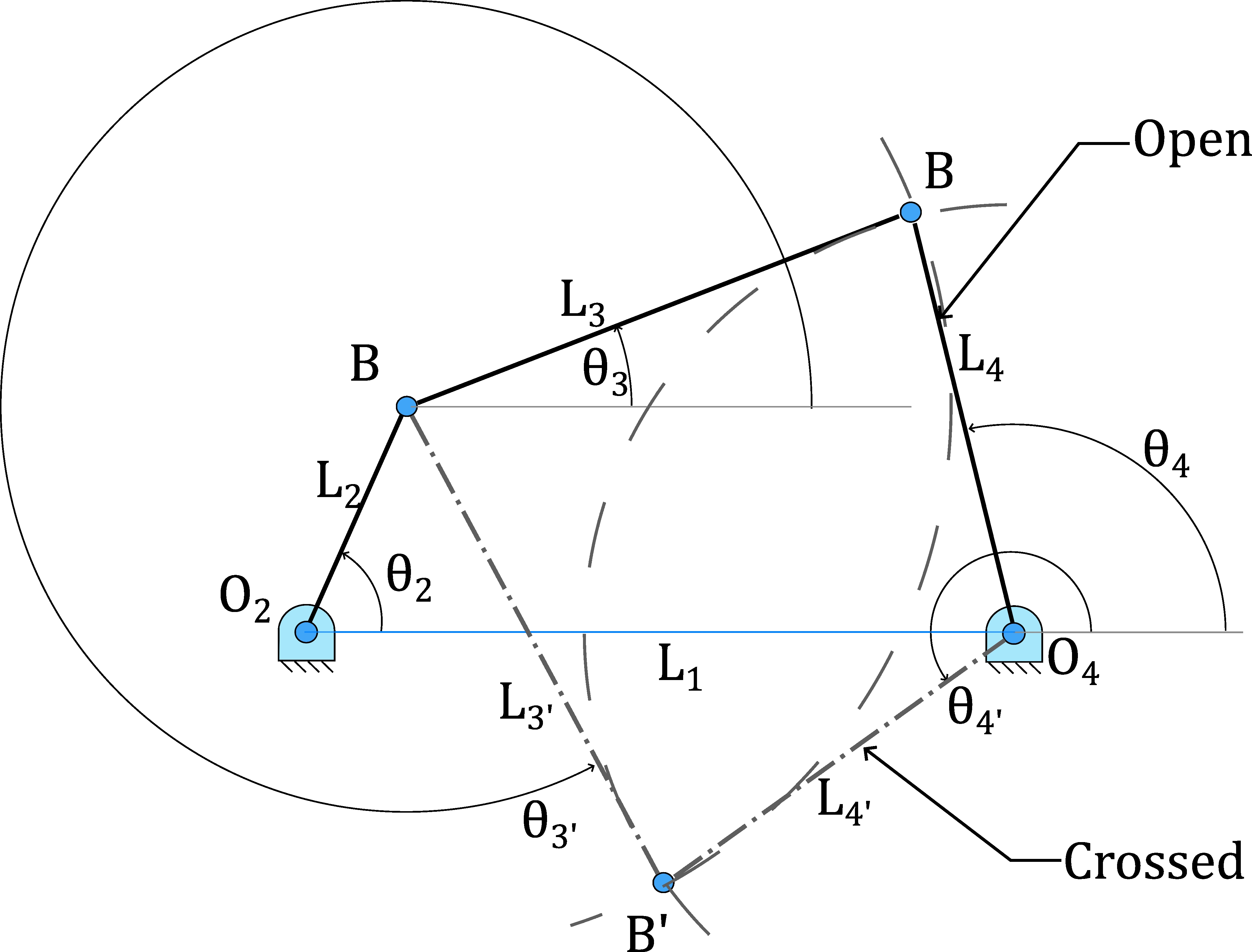
Close the loop: Here, the constraints of the remaining links are applied. For a four-bar linkage, point B must be simultaneously at a distance \(L_3\) from A and a distance \(L_4\) from \(O_4\).
A circle with center A and radius \(L_3\) is drawn.
Another circle with center \(O_4\) and radius \(L_4\) is drawn.
Identify the solutions: The intersection points of these two circles are the only two possible positions for joint B. This defines the two configurations or circuits of the mechanism (open and crossed). The designer must select the one that corresponds to the machine’s operation.
Analytical Method#
To obtain a precise solution and be able to calculate the position at any instant, the analytical method is used. This method is based on setting up a closed vector loop equation. For a four-bar linkage, it can be expressed by equating the two vector chains that connect the origin \(O_2\) to point B: \( \vec{L}_2 + \vec{L}_3 = \vec{L}_1 + \vec{L}_4 \) This vector equation is decomposed into two scalar equations (one for the horizontal components and one for the vertical components), as detailed in Example 2.1. This system of trigonometric equations is solved for the angular unknowns (\(\theta_3\) and \(\theta_4\)). The mathematical solution also yields two possible results, which correspond to the two configurations obtained graphically.