Lesson 4: Basic Concepts of Work and Energy Applied to Mechanisms#
Introduction: The Energy Approach#
In the previous lessons, we analyzed the dynamics of mechanisms using D’Alembert’s Principle. That method is based on the equilibrium of force and torque vectors, which, although complete, can be computationally costly and complex.
We now introduce an alternative and very powerful approach: the work-energy method. This method is based on scalar quantities (Work, Energy, Power) and is the fundamental tool for:
Directly relating forces, velocities, and displacements.
Analyzing the efficiency of a machine.
Sizing and selecting actuators (motors), since their main characteristic is the power they can deliver.
Learning objectives:#
By the end of this lesson, you will be able to:
Apply the energy balance to analyze the behavior of mechanisms.
Calculate the mechanical advantage and identify dead points in mechanisms.
Quantify losses due to passive resistances (friction in joints, rolling resistance).
Determine the efficiency of a mechanism and size the actuator it requires.
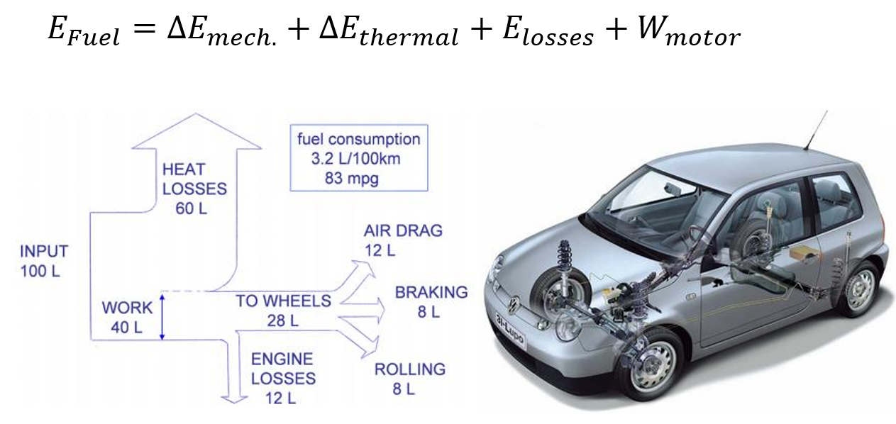
Example applied to a car:
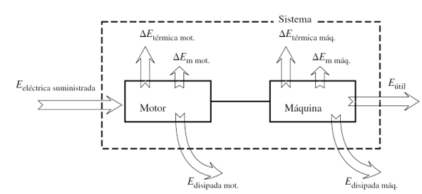
As this diagram illustrates, the energy balance is the key concept of this lesson. The “Supplied Energy” (generally from a motor) is not entirely converted into “Useful Energy” (the task we want to perform). In a real system, this input energy must:
Perform useful work.
Overcome the “Passive Resistances” (friction), which is dissipated as heat.
Change the “Mechanical Energy” (kinetic and potential) of the mechanism itself.
Throughout this lesson we will learn to quantify each of these parts using scalar tools that significantly simplify the analysis compared to vector methods.
Fundamental Concepts#
1. Work of a Force and a Torque#
Work is the measure of energy transfer due to the action of a force or a torque along a displacement.
Work of a Force (\(\vec{F}\)): It is the dot product of the force and the displacement of its application point. \(W_{12} = \int_{1}^{2} \vec{F} \cdot d\vec{r}\)
Work of a Torque (\(\vec{M}\)): It is the dot product of the torque and the angular displacement of the body. \(W_{12} = \int_{1}^{2} \vec{M} \cdot d\vec{\theta}\)
If the force (or torque) is constant, \(W = \vec{F} \cdot \Delta\vec{r}\) (or \(W = M \cdot \Delta\theta\) for torques).
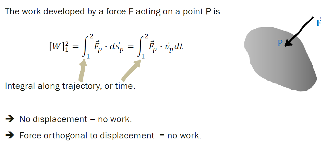
This image complements the formal definition of work. It is essential to understand that work is the integral of the dot product, which means that only the component of the force along the direction of the displacement (\(\vec{F} \cdot d\vec{s}\)), or the torque along the direction of rotation (\(T \cdot d\theta\)), does work. If a force is perpendicular to the displacement, its work is zero.
2. Power (\(P\))#
Power is the rate at which work is done; that is, the rate of energy transfer.
Power of a Force: \(P = \frac{dW}{dt} = \vec{F} \cdot \vec{v}\)
Power of a Torque: \(P = \frac{dW}{dt} = \vec{M} \cdot \vec{\omega}\)
In engineering, power is the key rating of a motor. A motor does not deliver “force,” it delivers power (a torque at a certain speed). The relations \(P = \vec{F} \cdot \vec{v}\) (dot product of force and velocity) and \(P = \vec{M} \cdot \vec{\omega}\) (dot product of torque and angular velocity) are fundamental and we will use them constantly for sizing actuators.
3. Kinetic Energy (\(E_c\))#
This is the energy associated with the motion of a body. For a rigid body in the plane (our case of study), it is decomposed into:
Translational Kinetic Energy: That of its center of gravity (CoG).
Rotational Kinetic Energy: About its CoG.
\(E_c = E_{c,\text{translation}} + E_{c,\text{rotation}} = \frac{1}{2} m v_G^2 + \frac{1}{2} I_G \omega^2\)
The total kinetic energy of a mechanism is the sum of the kinetic energies of all its moving links. The kinetic energy of a rigid body is the sum of the translational energy (\(E_{c,\text{translation}}\)) and the rotational energy (\(E_{c,\text{rotation}}\)). It is essential that this formula uses the velocity of the center of gravity (\(\vec{v}_G\)) and the moment of inertia about that same center of gravity (\(I_G\)).
4. Potential Energy (\(E_p\))#
This is the energy stored in a system due to its position or configuration. We are interested in two types:
Gravitational: \(E_p = mgh\) (due to the height \(h\) of the CoG).
Elastic (Springs): \(E_p = \frac{1}{2} k (L - L_0)^2\) (where \(k\) is the spring constant and \(L_0\) its free length).
Work-Energy Theorem#
This is the cornerstone of energy analysis. It states that the total work done by ALL forces (external and internal) acting on a system is equal to the change in its total kinetic energy.
\(\Delta E_c = W_{\text{total}}\) \(E_{c,2} - E_{c,1} = W_{1 \to 2}\)
We can decompose the total work (\(W_{\text{total}}\)) into:
\(W_{\text{driving}}\): (Positive) work done by the actuators.
\(W_{\text{resistant}}\): (Negative) work done by the useful loads.
\(W_{\text{conservative}}\): Work done by conservative forces (weight, springs). This work can be expressed as a change in Potential Energy: \(W_{\text{conservative}} = -\Delta E_p\).
\(W_{\text{passive}}\): (Negative) work dissipated by friction (passive resistances).
Rearranging, we obtain the General Energy Balance, the fundamental equation of this lesson:
\(W_{\text{driving}} + W_{\text{resistant}} + W_{\text{passive}} = \Delta E_c + \Delta E_p\)
This equation states that the net work done on a system must equal the change in its total mechanical energy.
Mechanical Advantage#
4.1. Ideal Mechanical Advantage (IMA) and the Principle of Virtual Work#
Principle of Virtual Work (PVW)#
For a system in quasi-static equilibrium (constant or zero velocity, hence \(\Delta E_c = 0\)), the virtual work (\(\delta W\)) of all forces and torques for a virtual displacement (\(\delta\vec{r}\) or \(\delta\vec{\theta}\)) is zero:
\(\delta W = \sum (\vec{F} \cdot \delta\vec{r}) + \sum (\vec{M} \cdot \delta\vec{\theta}) = 0\)
This principle is very powerful because it allows us to relate the input (driving) forces to the output (resistant) ones without needing to compute the internal reactions at the joints.
Definition of Ideal Mechanical Advantage#
Mechanical Advantage is a key design concept, indicating how much a mechanism “amplifies” the input force (or torque). It is defined as:
\(MA = \frac{\text{Output Force (Load)}}{\text{Input Force (Actuator)}}\)
Using the PVW in an ideal (frictionless) mechanism, the input virtual work equals the output virtual work, so the IMA is the ratio of velocities:
\(IMA = \frac{F_{\text{out}}}{F_{\text{in}}} = \frac{v_{\text{in}}}{v_{\text{out}}}\)
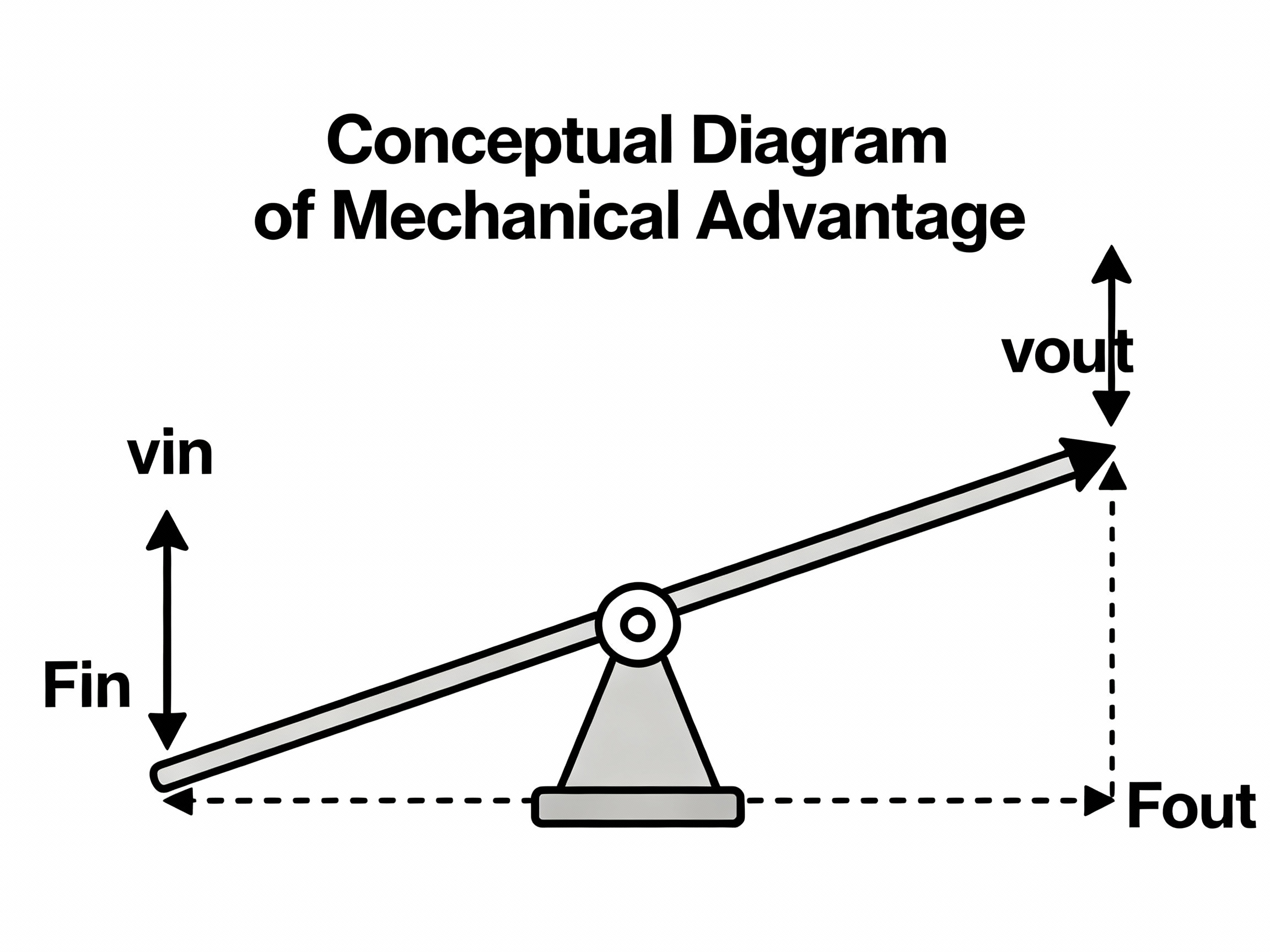
As we see in the lever image, this is the fundamental principle: if we want to amplify the force (\(F_{out} > F_{in}\)), we must accept a smaller output displacement (or a lower output velocity). It is a trade-off of force for velocity.
4.2. Variable Mechanical Advantage and Dead Points#
Mechanical Advantage (MA) is defined as the ratio between the output torque and the input torque (\(MA = M_{\text{out}} / M_{\text{in}}\)). In a four-bar mechanism, this MA is not constant; it varies with each position of the mechanism.
As can be deduced from the velocity polygon, the MA depends directly on the sines of the angles \(\beta\) and \(\gamma\) defined in the figure.
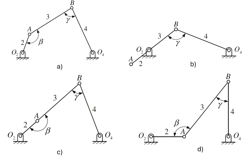
(Figure a) General Case: The mechanical advantage is directly proportional to the sine of \(\gamma\) (our transmission angle \(\mu\)) and inversely proportional to the sine of \(\beta\):
\(MA = \frac{M_{\text{out}}}{M_{\text{in}}} = \frac{\omega_{\text{in}}}{\omega_{\text{out}}} = \left(\frac{l_4}{l_2}\right) \frac{\sin(\gamma)}{\sin(\beta)}\)
(Figures b and c) Toggle Position (MA \(\to \infty\)): In figures (b) and ©, the input link (2) and the coupler (3) become aligned.
In Fig. (b), the angle \(\beta = 0^\circ\).
In Fig. ©, the angle \(\beta = 180^\circ\).
In both cases, \(\sin(\beta) = 0\). Since \(\sin(\beta)\) is in the denominator, the Mechanical Advantage becomes theoretically infinite (\(MA \to \infty\)). This is known as the toggle position. With a small input torque on link 2, an arbitrarily large resistant torque on link 4 can (ideally) be overcome.
(Figures b and c) Dead Point (MA \(\to 0\)): It is crucial to understand what happens if we swap the input and output at these same positions. If link 4 is now the input and link 2 the output, the new mechanical advantage \(MA_{\text{new}}\) is the reciprocal:
\(MA_{\text{new}} \propto \frac{\sin(\beta)}{\sin(\gamma)}\)
In positions (b) and ©, \(\sin(\beta) = 0\), so \(MA_{\text{new}} = 0\). The mechanism cannot transmit torque from link 4 to link 2. This is a dead point configuration for link 4.
(Figure d) Poor Transmission Angle (MA \(\to 0\)): Finally, figure (d) shows a position where the transmission angle \(\gamma\) (our \(\mu\)) is very small. Since \(MA \propto \sin(\gamma)\), if \(\gamma \to 0\), then the Mechanical Advantage tends to zero (\(MA \to 0\)). The mechanism is very inefficient at transmitting torque in this position.
In summary:
Dead points are positions where two links become aligned.
Depending on which link is the input, this alignment can result in either a Toggle Position (\(MA \to \infty\)) or a Dead Point (\(MA \to 0\)).
For good continuous-transmission design, the transmission angle \(\gamma\) (or \(\mu\)) should be kept from getting too small (generally \(\mu > 40^\circ\)).
Application Example: Toggle Position (Crusher)#
Here is an application example of the toggle position:
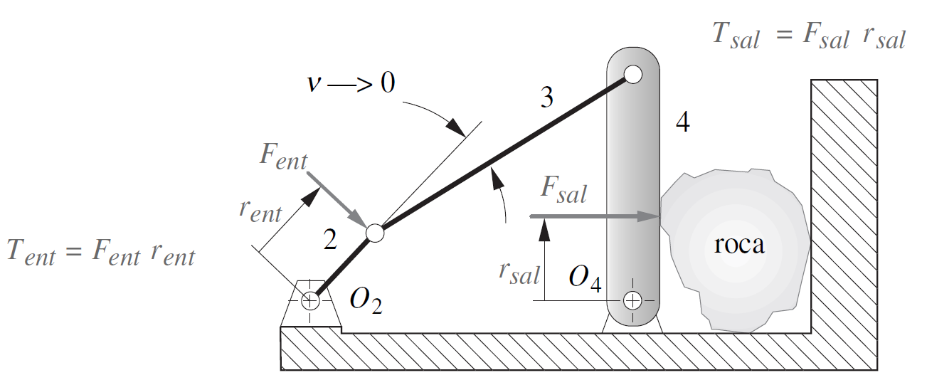
The crusher mechanism in the image is a perfect example of the use of the toggle position. The design is optimized so that, at the moment of maximum effort (when jaw 5 crushes the material), links 3 and 4 are nearly aligned.
This configuration corresponds to Figure © of the previous section, where \(\beta \to 180^\circ\). In this position, \(\sin(\beta) \to 0\).
Since the Mechanical Advantage is \(MA \propto 1/\sin(\beta)\), the \(MA\) tends to infinity. This allows the driving torque, applied on link 2, to generate an immense crushing force on link 5, overcoming the material’s high resistance with a moderately powered actuator.
Passive Resistances#
In a real mechanism, not all the input work is converted into useful work. Part of it is dissipated as heat due to friction. This is the passive work (\(W_{\text{passive}}\)), and it is the focus of our study in this lesson.
1. Friction in Revolute Joints (Bearings)#
Friction in a bearing (revolute joint) generates a friction torque \(\vec{M}_f\) that opposes the relative motion \(\vec{\omega}_{\text{rel}}\).
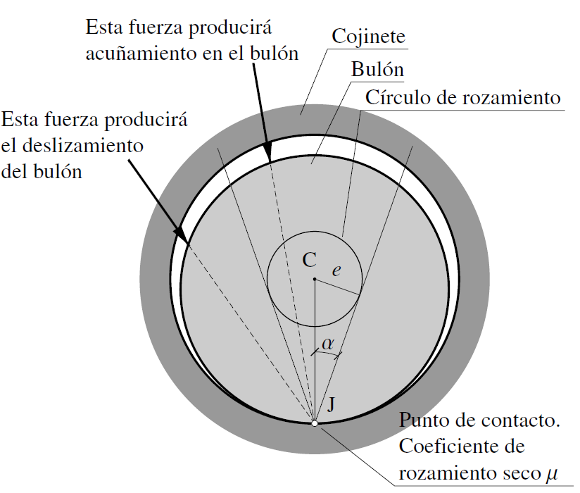
The figure illustrates the friction circle model:
Ideal Case (no friction): The reaction force \(R\) that the bearing exerts on the shaft would pass through the center.
Real Case (with friction): When the shaft rotates (here, \(\omega\) clockwise), it “climbs” the bearing surface. The total reaction \(R\) is deflected by an angle \(\phi\) (friction angle) and becomes tangent to a small circle, called the friction circle.
The radius of this circle is \(r_f = r \cdot \sin \phi\), where \(r\) is the shaft radius.
This off-center force \(R\) generates the friction torque \(M_f = R \cdot r_f\) that opposes the motion.
2. Friction in Prismatic Joints (Sliding)#
Friction in a guide (prismatic joint) generates a friction force \(\vec{F}_f\) opposed to the relative velocity \(\vec{v}_{\text{rel}}\).
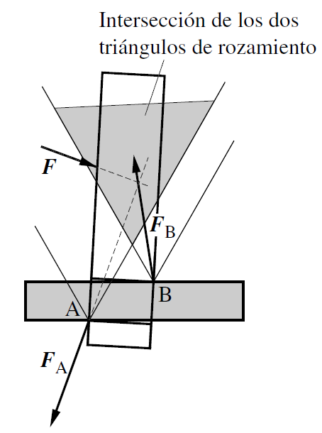
As the figure illustrates, the model is that of Coulomb’s law:
A body (slider) moves with velocity \(v\) along a guide.
The normal force \(N\) (which balances the weight \(P\)) produces a friction force \(F_f\) that opposes the motion.
The value of this force is \(F_f = \mu \cdot N\), where \(\mu\) is the (kinetic) coefficient of friction.
The dissipated power is \(P_f = F_f \cdot v\).
3. Rolling Resistance#
The last type of passive resistance we will study is rolling resistance. It is essential to understand that this phenomenon is not sliding friction, but an energy dissipation that occurs due to the deformation of the bodies in contact (the wheel and/or the road surface).
To understand its origin, we compare the ideal model (no deformation) with the real model (with deformation).
Figure 2. Rolling of a rigid cylinder on a rigid pavement.#
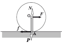
Description: This is the idealized physical model (“Rigid on Rigid”). Nothing deforms.
Reactions: The ground reaction occurs at a single point. The normal force (\(\vec{N}\)) is perfectly vertical and aligned with the weight (\(\vec{P}\)), so \(\vec{N} = -\vec{P}\).
Consequence: The normal force \(\vec{N}\) has no lever arm about the center of the wheel. There is no rolling resistance torque.
Figure 3. Rolling of a deformable cylinder on a rigid pavement.#
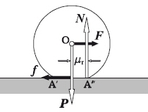
Description: This is the real model. It occurs when at least one of the bodies deforms (the image illustrates it as “Rigid on Deformable,” where the pavement sinks).
Reactions: Due to the deformation, the ground reaction is no longer a single point. The resultant of the vertical pressures (\(\vec{N}\)) shifts forward a distance \(b\).
The Resistant Torque: This force \(\vec{N}\) (which still balances the weight \(\vec{P}\)) now has a lever arm \(b\) about the center of the wheel. This creates the Rolling Resistance Torque (\(\vec{M}_{rr}\)): \(M_{rr} = N \cdot b = P \cdot b\)
The Coefficient (\(b\)): This distance \(b\) is the coefficient of rolling resistance (with units of length).
Resistance Force: For the wheel to advance at constant velocity, a traction force \(\vec{F}_{rr}\) must be applied to overcome this torque: \(\vec{F}_{rr} = \frac{\vec{M}_{rr}}{r} = \frac{P \cdot b}{r}\)
Efficiency (\(\eta\)) and Actuator Selection#
1. Efficiency#
Efficiency is the final concept that unifies everything above. It quantifies the effect of the passive resistances. It is the ratio between the useful power (or work) that leaves the mechanism and the power (or work) that enters it.
\(\eta = \frac{P_{\text{useful}}}{P_{\text{supplied}}} = \frac{P_{\text{out}}}{P_{\text{in}}}\)
Knowing that the input power must cover both the useful work and the friction losses (\(P_{\text{passive}}\)): \(P_{\text{supplied}} = P_{\text{useful}} + P_{\text{passive}}\)
Therefore, the efficiency is always less than 1: \(\eta = \frac{P_{\text{useful}}}{P_{\text{useful}} + P_{\text{passive}}} < 1\)
Efficiency is crucial for correctly sizing a real motor: the motor must be able to supply \(P_{\text{supplied}}\), not just \(P_{\text{useful}}\).
2. Torque-Speed Characteristic Curves and Motor Selection#
Knowing the required power (computed with the efficiency) is the first step. The second step is selecting a suitable motor. For this, torque-speed characteristic curves are used.
The characteristic curve describes the torque required for the machine to run at constant speed (zero acceleration).
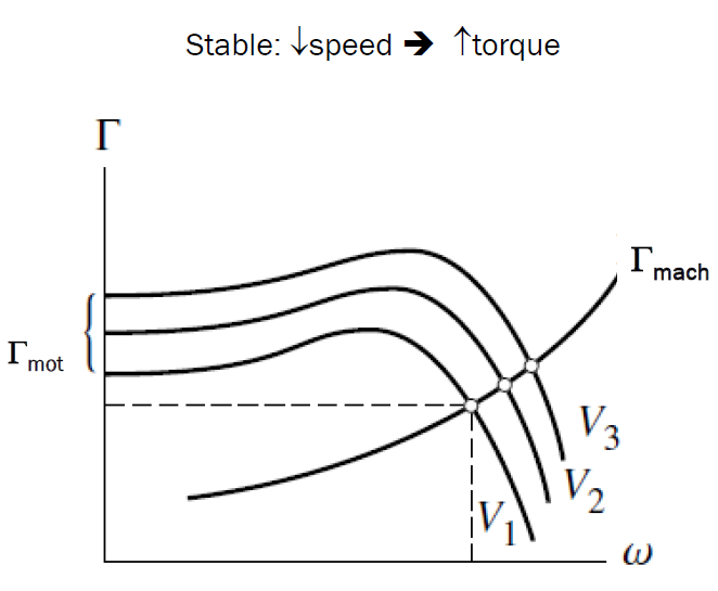
As shown in the graph, two types of curves are overlaid:
Motor torque (\(M_{\text{mot}}\)): The torque the motor supplies. Several curves are usually shown for different supply voltage values (\(V\)).
Machine resistant torque (\(M_{\text{mach}}\)): The torque the machine demands (opposing the motion) to overcome the useful load and all its passive resistances.
The intersection points are the equilibrium points. They define the operating speed at which the system will run for a given motor voltage.
Lesson Summary#
In this lesson we introduced the energy approach for analyzing mechanisms, which complements and simplifies the vector-based dynamic approach seen previously. The key concepts you should master are:
General Energy Balance: Relates the work of the driving and resistant forces to the changes in the mechanical energy of the system.
Mechanical Advantage: Quantifies the force (or torque) amplification provided by a mechanism. It varies with the configuration and is critical in design.
Dead Points and Toggle Positions: Special configurations where the MA tends to zero or infinity, respectively. They must be taken into account in the design depending on the application.
Passive Resistances: Friction in revolute and prismatic joints, and rolling resistance. These losses reduce efficiency and must be included when computing the required power.
Efficiency: Quantifies the total losses of the system and is essential for correctly sizing the actuator.
Actuator Selection: Carried out using torque-speed characteristic curves, identifying the equilibrium points between the available motor torque and the demanded resistant torque.
These concepts are fundamental for the design and analysis of any mechanical system in engineering practice.