Example 5.01: Dynamic Balancing#
Problem Statement#
Determine the mass (\(m_{c1}\) and \(m_{c2}\)) and the placement angle (\(\theta_{c1}\) and \(\theta_{c2}\)) of two correction masses. These masses are placed in correction planes A (at \(d=0 \,\text{cm}\)) and B (at \(d=6 \,\text{cm}\)) respectively, both at a radius \(r_c = 2 \,\text{cm}\).
The goal is to dynamically balance the system shown in the figure, which rotates at constant speed.
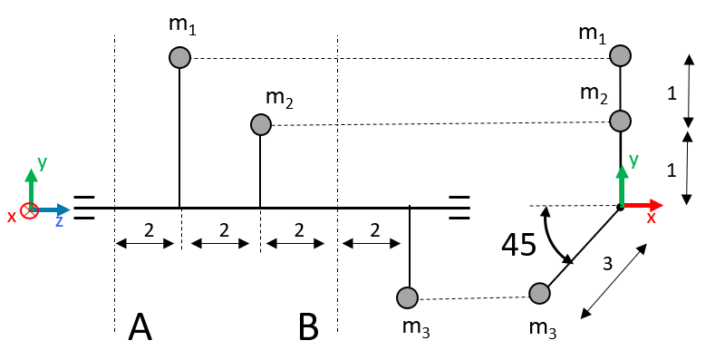
Data for the existing unbalance masses:
\(m_1 = 200 \,\text{g}\)
\(m_2 = 400 \,\text{g}\)
\(m_3 = 300 \,\text{g}\)
(Note: the radii and axial distances of these masses are defined in the data section. Units are kept consistent in \(\text{g}\) and \(\text{cm}\) throughout the calculation.)
1. Known Data#
First, we define the symbolic variables for our unknowns and the known problem data (masses, radii, angles, and axial distances).
clear; clc; close all
syms mc1 mc2 thc1 thc2 %(Unknowns: correction masses 1 and 2, and their angles)

% --- KNOWN DATA ---
% Existing unbalance masses
m1=200; m2=400; m3=300; % (g)
% Radii of the existing masses
r1=2; r2=1; r3=3;       % (cm) - consistent units (g*cm)
% Radii where the correction masses will be placed
rc1=2; rc2=2;            % (cm)
% Axial positions (distances along the Z axis)
% IMPORTANT: correction plane 1 (A) is taken as the origin (moment plane).
d_c1 = 0;   % Moment origin (Plane A)
d1   = 2;
d2   = 4;
d_c2 = 6;   % Correction plane 2 (Plane B)
d3   = 8;
% Angles of the existing masses
th1=deg2rad(90); th2=deg2rad(90); th3=deg2rad(225);
2. Setting up the Vector Equations#
We use the Unbalance Vectors (\(\vec{U} = m\vec{r}\)). The angular speed term (\(\omega^2\)) cancels out of the balance equations, so we work directly with the products \(m \cdot r\).
% Unbalance vectors (U = m*r) of the CORRECTION masses (Unknowns)
% Format: [Ux, Uy, Uz]
U_c1=[mc1*rc1*cos(thc1), mc1*rc1*sin(thc1), 0];
U_c2=[mc2*rc2*cos(thc2), mc2*rc2*sin(thc2), 0];

% Unbalance vectors (U = m*r) of the EXISTING masses (Data)
U1=[m1*r1*cos(th1), m1*r1*sin(th1), 0];
U2=[m2*r2*cos(th2), m2*r2*sin(th2), 0];
U3=[m3*r3*cos(th3), m3*r3*sin(th3), 0];
Equation 1: Force Balance (\(\sum \vec{U} = 0\))#
The vector sum of all unbalances (existing + correction) must be zero.
eq_Forces = U_c1 + U_c2 + U1 + U2 + U3 == 0;
Equation 2: Moment Balance (\(\sum (\vec{d} \times \vec{U}) = 0\))#
Moments are taken about correction Plane 1 (at \(d_{c1} = 0\)). The moment \(\vec{M}_{c1}\) is ZERO, which simplifies the solution.
M1   = cross([0 0 d1],   U1);
M2   = cross([0 0 d2],   U2);
M3   = cross([0 0 d3],   U3);
M_c2 = cross([0 0 d_c2], U_c2);
% M_c1 = cross([0 0 d_c1], U_c1) == 0; (which is why it is not included)

eq_Moments = M_c2 + M1 + M2 + M3 == 0;
3. Solving the Symbolic System#
We solve the system of 4 scalar equations (X and Y components of forces and moments) for the 4 unknowns (\(m_{c1}, m_{c2}, \theta_{c1}, \theta_{c2}\)).
sol = solve([eq_Forces(1:2), eq_Moments(1:2)], mc1, mc2, thc1, thc2);
4. Extracting and Correcting the Results#
The solve command returns mathematical solutions. A negative mass (e.g. -50g @ 300°) is mathematically correct, but physically we interpret it as a positive mass (+50g) placed 180° away.
% Select one of the numerical solutions (e.g., #2).
idx_sol = 2;

mc1_sol = double(sol.mc1(idx_sol));
thc1_sol_rad = double(sol.thc1(idx_sol));

mc2_sol = double(sol.mc2(idx_sol));
thc2_sol_rad = double(sol.thc2(idx_sol));

% --- NEGATIVE MASS CORRECTION ---
if mc1_sol < 0
    mc1_sol = -mc1_sol;
    thc1_sol_rad = thc1_sol_rad + pi;
end

if mc2_sol < 0
    mc2_sol = -mc2_sol;
    thc2_sol_rad = thc2_sol_rad + pi;
end

% --- ANGLE NORMALIZATION ---
thc1_sol_deg = mod(rad2deg(thc1_sol_rad), 360);
thc2_sol_deg = mod(rad2deg(thc2_sol_rad), 360);
5. Printing the Final Results#
fprintf('--- Balancing Results (Symbolic Method) ---\n');
fprintf('Plane A (at d=%g cm):\n', d_c1);
fprintf('  Correction Mass (mc1): %g (g)\n', mc1_sol);
fprintf('  Correction Angle (thc1): %g (degrees)\n', thc1_sol_deg);
fprintf('-----------------------------------------------------\n');
fprintf('Plane B (at d=%g cm):\n', d_c2);
fprintf('  Correction Mass (mc2): %g (g)\n', mc2_sol);
fprintf('  Correction Angle (thc2): %g (degrees)\n', thc2_sol_deg);
Balancing Results (Symbolic Method)#
Correction Mass 1 (\(m_{c1}\)): 14.0117 (kg) Correction Angle 1 (\(\theta_{c1}\)): 277.507 (degrees) Correction Mass 2 ( \(m_{c2}\)): 5.37412 (kg) Correction Angle 2 (\(\theta_{c2}\)): 70.0848 (degrees)