
D’Alembert’s principle#
Loads on a mechanism#
Forces are transmitted through the links of a mechanism at their contact points (the joints). The links are subjected to:
Their own weight.
External loads: useful or resisting forces (for instance, the cutting resistance on the tool of a shaper), spring forces, gas pressure in an engine…
The input torque or the actuator forces.
Passive resistances (friction), see Friction forces.
The reactions at the joints, which transmit loads from one link to another.
The effects of the accelerations of the links, treated as inertia loads.
Each force is a vector, defined by its magnitude, its line of action and sense, and its point of application (for a rigid body, it is enough to know the line of action, since the force can slide along it).
Statement#
We start from the Newton-Euler equations of a rigid body (see Rigid body dynamics):
If we move the right-hand side terms to the left and interpret them as one more force and one more moment, called the inertia force \(\vec{F}_{in}\) and the inertia torque \(\vec{M}_{in}\):
the equations become those of statics:
If the inertia forces and torques are added as acting forces to a moving body, the body is in static equilibrium (dynamic equilibrium):
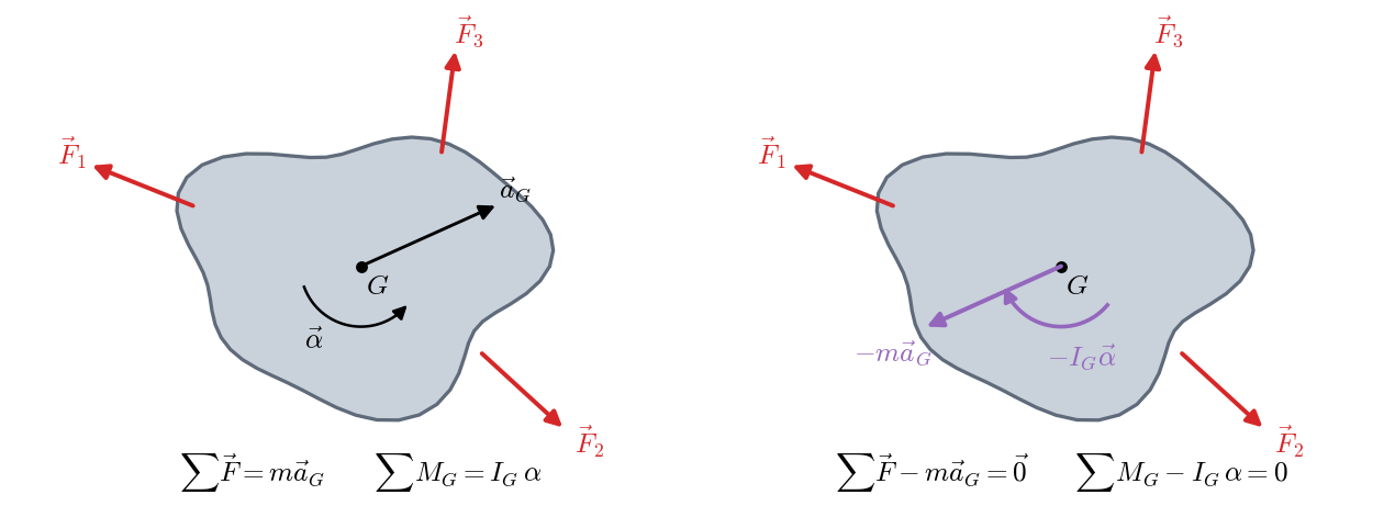
Inertia loads are fictitious: no body exerts them, so they have no reaction. They are a device that lets us treat a dynamic problem with all the tools of statics:
The inertia force is opposite to the acceleration of \(G\), and it is applied at \(G\).
The inertia torque is opposite to the angular acceleration.
Once they are added, the sum of moments is zero about any point, not just about \(G\). This is a great practical advantage: we can take moments about a joint to get rid of the unknown reactions passing through it.
In the notation of the slides on graphical methods, the inertia force is also called \(\vec{J} = -m\vec{a}_G\) and the inertia torque \(M_G = -I_G\,\alpha\).
Why is the inertia force applied at \(G\), and why is the torque \(-I_G\alpha\)?
Each element \(dm\) of a planar link has an acceleration \(\vec{a}_K = \vec{a}_G + \vec{a}^n_{KG} + \vec{a}^t_{KG}\), and its elementary inertia force is \(d\vec{J} = -\vec{a}_K\, dm\). Integrating over the whole link:
Since \(\vec{a}^n_{KG} = -\omega^2\, \vec{GK}\) and \(\vec{a}^t_{KG} = \vec{\alpha}\times\vec{GK}\), the last two integrals are proportional to \(\int_V \vec{GK}\,dm\), the first moment of mass about the center of mass, which is zero. This leaves \(\vec{J} = -m\,\vec{a}_G\).
Taking moments about \(G\), \(d\vec{M}_G = \vec{GK}\times d\vec{J}\). The term with \(\vec{a}_G\) vanishes again because the first moment of mass is zero; the one with \(\vec{a}^n_{KG}\), because it is parallel to \(\vec{GK}\); and the tangential one gives:
Equivalent inertia force#
In a planar link, the inertia force \(\vec{J}\) (applied at \(G\)) and the inertia torque \(M_G\) can be replaced by a single force \(\vec{J}' = \vec{J}\) shifted parallel to itself a distance \(h\), so that its moment about \(G\) equals \(M_G\):
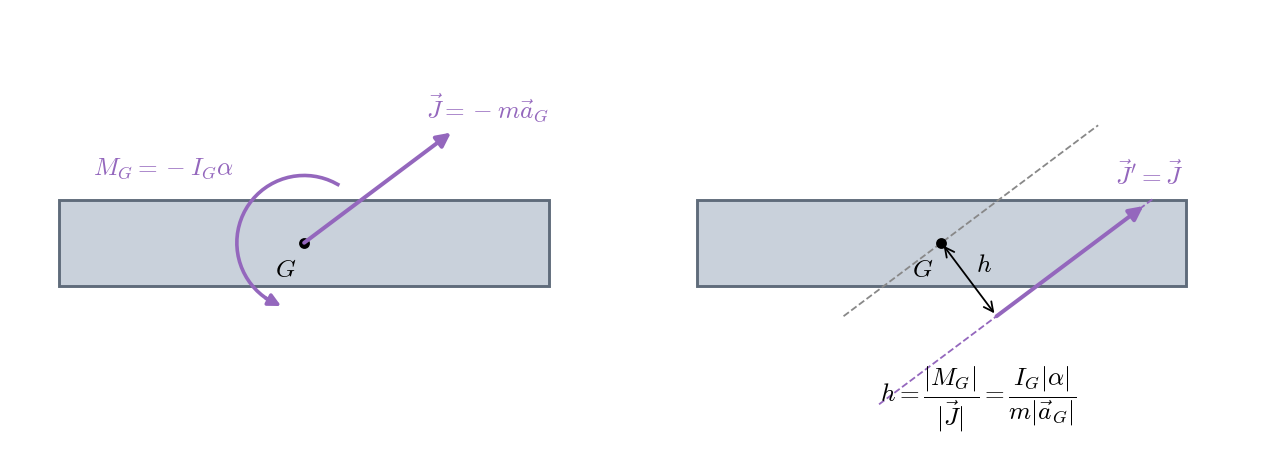
The side to shift it to is chosen so that the moment of \(\vec{J}'\) about \(G\) has the same sense as \(M_G\), that is, opposite to \(\alpha\). This single force is very useful in graphical methods (see Graphical methods), because it turns a link with an inertia force and torque into a link with one more force.
Particular cases:
Link in translation (\(\alpha = 0\)): there is only an inertia force, applied at \(G\) (\(h = 0\)).
Link rotating about its center of mass (\(\vec{a}_G = \vec{0}\)): there is only an inertia torque.
Link rotating at constant speed about a fixed point \(O\): \(\alpha = 0\) and the inertia force is the centrifugal force \(m\,\omega^2\, |OG|\), pointing from \(O\) towards \(G\).
Quasi-static analysis#
If a mechanism moves slowly (low or zero velocities and accelerations), the inertia loads are negligible compared with the external loads, and the problem reduces to static equilibrium:
This is the case of a robotic gripper squeezing a part (see Example 3.1: Robotic gripper (quasi-static analysis)), of a press or of a locking mechanism. For a mechanism to be in equilibrium, it is necessary and sufficient that each of its links is in equilibrium.
Superposition principle#
In linear problems (without friction, which introduces inequalities), the effect of several forces acting on a mechanism is the sum of the effects of each one separately. If two force systems each keep the mechanism in equilibrium, so does their sum.
Therefore, the complete kinetostatic analysis of a mechanism can be split into:
Static analysis: reactions and input torque due to the external loads alone.
Dynamic analysis: reactions and input torque due to the inertia loads alone.
Vector sum of both results, link by link.
This principle is especially useful in graphical methods, where each force polygon can only solve for two unknowns. For each force or inertia load acting only on link \(i\), all the reactions of the mechanism follow from a simple problem, and the total solution is the sum of the partial ones:
A complete example is in Example 3.6: Inertia forces in a four-bar linkage (graphical method). In a reciprocating engine, for instance, the effective torque at the crankshaft is the difference between the torque produced by the gas (static analysis) and the torque needed to accelerate the masses (dynamic analysis).
Solution procedure#
To compute the reactions and the input torque of a mechanism with known motion:
Solve the complete kinematics: accelerations of the centers of mass \(\vec{a}_{G_i}\) and angular accelerations \(\alpha_i\) of all moving links (lesson 2).
Add the inertia loads of each link: \(\vec{F}_{in,i} = -m_i\vec{a}_{G_i}\) at \(G_i\) and \(M_{in,i} = -I_{G_i}\alpha_i\). They are proportional to the accelerations and opposite to them.
Write the static equilibrium of all links, separately, with their free-body diagrams. The whole mechanism will then be in dynamic equilibrium.
Step 3 can be done analytically, by writing and solving a system of equations (Analytical force method), or graphically, with force polygons (Graphical methods).