
Example 2.2: Kinematic analysis of a slider-crank mechanism#
Position analysis#
The figure shows a slider-crank mechanism. For the instant when the crank forms an angle \(\theta_2 = 30^{\circ}\) with the horizontal, calculate the position of the slider and the angle that link 3 forms with the horizontal.
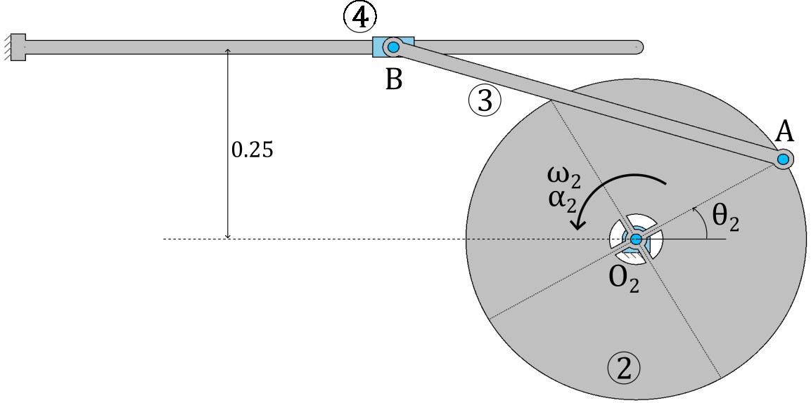
Data:
Link lengths, in meters: \(\overline{O_2 A} = 0.25;\,\overline{AB} = 0.6;\,y_B = 0.25;\)
Position analysis: graphical method#
The objective is to construct the mechanism’s configuration to scale for the instant \(\theta_2 = 30^\circ\) and measure the position unknowns: the horizontal coordinate of the slider (\(x_B\)) and the angle of the coupler (\(\theta_3\)).
Construction Data:#
Link 2 (Crank): \(L_2 = \overline{O_2A} = 0.25 \text{ m}\)
Link 3 (Coupler): \(L_3 = \overline{AB} = 0.6 \text{ m}\)
Slider Axis: The slider moves on a horizontal line at a constant height \(y_B = 0.25 \text{ m}\).
Input Angle: \(\theta_2 = 30^\circ\).
Construction Procedure:#
Establish the origin: The fixed pivot \(O_2\) is placed at the coordinate origin (0,0).
Position the crank (Link 2): From \(O_2\), link 2 is drawn with its length \(L_2 = 0.25 \text{ m}\) and the input angle \(\theta_2 = 30^\circ\). The end of this vector is the position of joint A.
Draw the slider guide: The horizontal line that defines the path of slider B is drawn. This line is at a constant height \(y = 0.25 \text{ m}\).
Locate joint B (Loop closure):
Coupler Constraint: Point B must be at a distance \(L_3 = 0.6 \text{ m}\) from A. Geometrically, this is a circle with center A and radius 0.6.
Slider Constraint: Point B must lie on the line \(y = 0.25\).
Resolve configuration ambiguity: The intersection of the circle (center A, radius \(L_3\)) and the line (\(y=0.25\)) yields two possible solutions for point B. The one corresponding to the configuration shown in the problem figure must be chosen.
Measurement of results: With the mechanism fully drawn, the desired quantities are measured directly from the graphical software:
Coordinates of point B: \((x_B, y_B)\).
Angle of the coupler, \(\theta_3\): The angle of the segment AB with the horizontal.
Position analysis: analytical method#
The objective is to find expressions for the unknowns (\(x_B\) and \(\theta_3\)) as a function of the known parameters.
Vector Loop Formulation#
We model the mechanism as an open vector chain. The position of point B can be expressed starting from the origin \(O_2\): \( \vec{R}_B = \vec{R}_A + \vec{R}_{AB} \) Where:
\(\vec{R}_A = L_2(\cos\theta_2 \hat{i} + \sin\theta_2 \hat{j})\)
\(\vec{R}_{AB} = L_3(\cos\theta_3 \hat{i} + \sin\theta_3 \hat{j})\)
\(\vec{R}_B = x_B \hat{i} + y_B \hat{j}\) (with \(y_B\) constant)
We decompose the vector equation into its scalar components (x and y):
x-component: \( x_B = L_2\cos\theta_2 + L_3\cos\theta_3 \quad (\text{Equation 1}) \)
y-component: \( y_B = L_2\sin\theta_2 + L_3\sin\theta_3 \quad (\text{Equation 2}) \)
We have a system of two equations with two unknowns: \(\theta_3\) and \(x_B\).
Solving for \(\theta_3\) and \(x_B\)#
Solve for \(\theta_3\): From Equation 2, we can solve for \(\sin\theta_3\): \( \sin\theta_3 = \frac{y_B - L_2\sin\theta_2}{L_3} \) This will give us two possible values for \(\theta_3\), since \(\theta_{3,2} = 180^\circ - \theta_{3,1}\). We must choose the solution that corresponds to the configuration in the drawing. Once \(\sin\theta_3\) is known, we can find \(\cos\theta_3 = \pm\sqrt{1 - \sin^2\theta_3}\), where the sign depends on the quadrant in which \(\theta_3\) lies.
Solve for \(x_B\): Once we have the correct value of \(\theta_3\) (and therefore, of \(\cos\theta_3\)), we substitute it into Equation 1 to find the position of the slider: \( x_B = L_2\cos\theta_2 + L_3\cos\theta_3 \)
Numerical Calculation for the Example#
The calculation is performed for the two possible configurations.
Initial Data:
Lengths: \(L_2=0.25 \text{ m}, L_3=0.6 \text{ m}\)
Vertical position of the slider: \(y_B = 0.25 \text{ m}\)
Input angle: \(\theta_2 = 30^\circ\)
Calculation of \(\theta_3\): Using Equation 2: \( \sin\theta_3 = \frac{0.25 - 0.25\sin(30^\circ)}{0.6} = \frac{0.25 - 0.25 \cdot 0.5}{0.6} = \frac{0.125}{0.6} \approx 0.2083 \) This gives two possible solutions for \(\theta_3\):
Solution 1: \(\theta_{3,1} = \arcsin(0.2083) \approx 12.02^\circ\). This corresponds to the configuration in the figure.
Solution 2: \(\theta_{3,2} = 180^\circ - 12.02^\circ = 167.98^\circ\). This corresponds to the other possible configuration of the mechanism.
Calculation of \(x_B\) (for Solution 2): The second solution for \(\theta_3\) is chosen. First, we calculate the cosine for this angle: \( \cos(167.98^\circ) \approx -0.9781 \) Now, we use Equation 1: \( x_B = 0.25\cos(30^\circ) + 0.6\cos(167.98^\circ) = 0.25 \cdot 0.866 + 0.6 \cdot (-0.9781) \) \( x_B = 0.2165 - 0.5868 = -0.3703 \text{ m} \)
Final Position Results (Solution 2):
Coupler angle: \(\mathbf{\theta_3 = 167.98^\circ}\)
Slider position: \(\mathbf{x_B = -0.3703 \text{ m}}\)
Velocity analysis#
At the instant when the crank forms an angle \(\theta_2 = 30^{\circ}\) with the horizontal, its angular velocity is \(\vec{\omega}_2 = 1\hat{k}\) rad/s, and its acceleration is \(\vec{\alpha}_2 = 1\hat{k}\) rad/s². Calculate the velocity of the slider and the angular velocity of link 3.
Data:
Link lengths, in meters: \(\overline{O_2 A} = 0.25;\, \overline{AB} = 0.6;\, y_B = 0.25\). Angle of link 3 with the horizontal, from the position analysis: \(\theta_3 = 167.98^{\circ}\).
Resolution (Calculations in Matlab)#
For this example, we will perform the calculations using Matlab. We start by creating variables for the given data:
clear, clc
O2A = 0.25; AB = 0.6;
th2 = 30; th3 = 167.98;
w2 = [0 0 1]; af2 = [0 0 1];
The mechanism has one degree of freedom, corresponding to \(\vec{\omega}_2\). We use this known data to calculate the velocity of point A:
\(\vec{v}_A = \vec{\omega}_2 \times \vec{r}_{O2A}\)
From the geometric data, we calculate \(\vec{r}_{O2A}\):
rO2A = O2A * [cosd(th2) sind(th2) 0];
Therefore,
\(\vec{v}_A = 1\hat{k} \times (0.2165\hat{i} + 0.125\hat{j}) = -0.125\hat{i} + 0.2165\hat{j}\)
vA = cross(w2, rO2A);
Next, we focus on point B. Analyzing it as part of link 3, we can establish the relative velocity equation between A and B:
\(\vec{v}_{B3} = \vec{v}_A + \vec{v}_{B/A}\)
with \(\vec{v}_A\) known and \(\vec{v}_{B/A} = \vec{\omega}_3 \times \vec{r}_{AB}\), where we know the direction but not the magnitude of \(\vec{\omega}_3\).
syms w3k real
w3 = [0 0 w3k];
rAB = AB * [cosd(th3) sind(th3) 0];
vB_A = cross(w3, rAB);
vB3 = vA + vB_A;
Now we analyze point B as part of link 4 (the slider). Since it’s a slider, we know its direction must be along the sliding axis, which is horizontal in this case:
\(\vec{v}_{B4} = v_B\hat{i}\)
syms vBi real
vB4 = [vBi 0 0];
Since there is a revolute joint at B, we can equate the two expressions:
sol_v1 = solve(vB3 == vB4, w3k, vBi);
w3k = double(sol_v1.w3k);
vBi = double(sol_v1.vBi);
fprintf('w3k=%0.3f vBi=%0.3f\n', w3k, vBi)
w3k=0.369 vBi=-0.171
Velocity Cinema#
The velocity cinema for this example is not provided, but it can be created using the same principles demonstrated in previous examples.
Acceleration analysis#
At the instant when the crank forms an angle \(\theta_2 = 30^{\circ}\) with the horizontal, its angular velocity is \(\vec{\omega}_2 = 1\hat{k}\) rad/s, and its acceleration is \(\vec{\alpha}_2 = 1\hat{k}\) rad/s². Calculate the acceleration of the slider and the angular acceleration of link 3.
Data:
Link lengths, in meters: \(\overline{O_2 A} = 0.25;\, \overline{AB} = 0.6;\, y_B = 0.25\). Angle of link 3 with the horizontal (from position analysis): \(\theta_3 = 167.98^{\circ}\), and its angular velocity \(\vec{\omega}_3 = 0.369\) rad/s.
Resolution (Calculations in Matlab)#
The procedure for calculating the mechanism’s accelerations is similar to that for velocities. We start with point A as we have information about it. We calculate \(\vec{a}_A\) from its normal and tangential components:
\(\vec{a}_A = \vec{a}_A^n + \vec{a}_A^t = \vec{\omega}_2 \times (\vec{\omega}_2 \times \vec{r}_{O2A}) + \vec{\alpha}_2 \times \vec{r}_{O2A}\)
aA = cross(w2, cross(w2, rO2A)) + cross(af2, rO2A);
Now, analyzing point B as part of link 3, we have:
\(\vec{a}_{B3} = \vec{a}_A + \vec{a}_{B/A}\)
which, by decomposing, gives:
\(\vec{a}_{B3} = \vec{a}_A + \vec{a}_{B/A}^n + \vec{a}_{B/A}^t\)
where the acceleration of A is known, and we can express the components of the relative acceleration from the available information:
For \(\vec{a}_{B/A}^n\), everything is known. Therefore: \(\vec{a}_{B/A}^n = \vec{\omega}_3 \times (\vec{\omega}_3 \times \vec{r}_{AB})\)
aB_An = cross(w3, cross(w3, rAB));
For \(\vec{a}_{B/A}^t\), we can operate and express it in terms of the unknown \(\vec{\alpha}_3\), of which we only know its direction: \(\vec{a}_{B/A}^t = \vec{\alpha}_3 \times \vec{r}_{AB}\)
syms af3k real
af3 = [0 0 af3k];
aB_At = cross(af3, rAB);
Which leaves us with:
aB3 = aA + aB_An + aB_At;
On the other hand, if we consider point B as part of link 4, we have:
\(\vec{a}_{B4} = a_B\hat{i}\)
syms aBi real
aB4 = [aBi 0 0];
Finally, if we equate both expressions, we have:
sol_ac1 = solve(aB3 == aB4, af3k, aBi);
af3k = double(subs(sol_ac1.af3k));
aBi = double(subs(sol_ac1.aBi));
fprintf('af3k=%0.3f aBi=%0.3f\n', af3k, aBi)
af3k=0.127 aBi=-0.277
Acceleration Cinema#
The acceleration cinema for this example is not provided, but it can be created using the same principles demonstrated in previous examples.