
Example 2.9: Bicycle suspension#
The mechanism in the photo (dimensions in centimeters) shows the rear suspension of a bicycle (adapted from the January 2023 exam). Find:
The number of degrees of freedom.
The velocity of point \(A\), using the analytical method.
The angular accelerations of all links and the acceleration of the rear wheel center, \(C\).
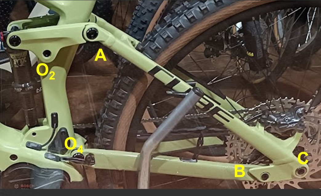
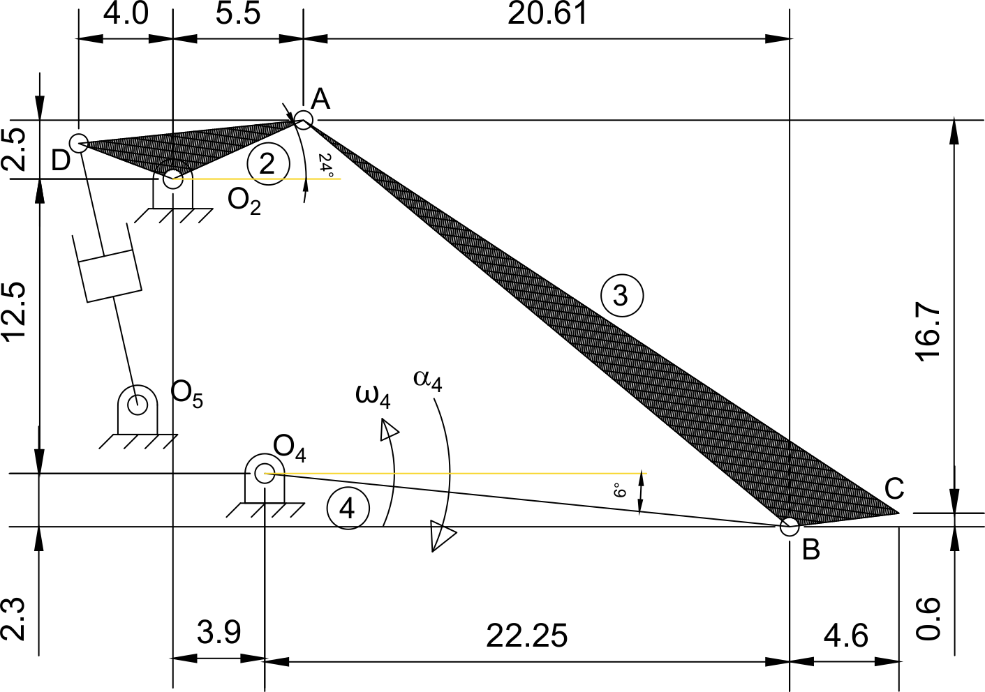
Data: \(\omega_4= 1~rad/s\) counterclockwise; \(\alpha_4= 2~rad/s^2\) clockwise. Any other dimension needed can be measured from the figure.
Solution
1. Degrees of freedom
The spring-damper unit \(O_5\)-\(D\) neither adds nor removes degrees of freedom, so it may or may not be counted. If it is not counted:
\(N=4\) bodies (counting the ground as a body).
\(p_I=4\) revolute joints (\(O_2\): 1-2, \(O_4\): 1-4, \(A\): 2-3 and \(B\): 3-4).
\(p_{II}=0\), since there are no two-d.o.f. joints.
Applying Grübler’s formula: \(G=3(N-1)-2 p_I - p_{II} = 3 \cdot 3 - 2 \cdot 4 = 1\) d.o.f.
If the spring-damper unit is counted, it consists of two bodies sliding on each other: Body 5 (lower half) and Body 6 (upper half, the one attached to Body 2). Then:
\(N=6\) bodies.
\(p_I=7\): six revolute joints (1-2, 1-4, 2-3, 3-4, 2-6 and 1-5) and one prismatic joint (5-6).
\(p_{II}=0\).
This gives \(G = 3 \cdot 5 - 2 \cdot 7 = 1\) d.o.f., matching the previous result, as expected.
2. Velocity of point \(A\)
Since this is a one-d.o.f. mechanism, a single velocity (and acceleration) input is enough to solve for all the others. The strategy is to find a loop that covers all the bodies of the kinematic chain to be analyzed, write the relative-motion equations of the points along that loop, and solve the resulting system. The loop will be \(O_4\)-\(B\)-\(A\)-\(O_2\), with the following position vectors (in cm, measured from the figure):
The velocity equations along the loop are:
The first one can be evaluated directly: \(\vec{v}_B = (1\,\hat{k}) \times (22.246\,\hat{i} - 2.259\,\hat{j}) = 2.259\,\hat{i} + 22.246\,\hat{j}~(cm/s)\). Substituting the other two into the third:
which is a system of two equations with two unknowns, whose solution is:
The requested velocity is therefore:
3. Accelerations
We write the equivalent system with the rigid-body acceleration equations along the same loop:
where \(\vec{a}_B = -26.76\,\hat{i} - 42.23\,\hat{j}~(cm/s^2)\) is known and the unknowns are \(\alpha_2\) and \(\alpha_3\). Solving:
Point \(C\) is not part of the loop used to set up the system, but once \(\omega_3\) and \(\alpha_3\) are known, its acceleration follows directly from the equation of rigid body 3:
The following MATLAB code solves the problem using the Symbolic Math Toolbox:
clear, clc, close all

% Geometric data (cm):
rO2A=[5.529 2.499 0];
rO4B=[22.246 -2.259 0];
rAB=[20.609 -17.248 0];
rBC=[4.6 0.6 0];

% Known inputs:
w4=[0 0 1];
af4=[0 0 -2];

% Symbolic unknowns:
syms w2M w3M real

% Velocities:
w3=[0 0 w3M];
w2=[0 0 w2M];
vA=cross(w2,rO2A);
vB=cross(w4,rO4B);

eq1= vB==vA+cross(w3,rAB);

sol1=solve(eq1,[w3M,w2M]);
w2M=eval(sol1.w2M);
w3M=eval(sol1.w3M);
w3=[0 0 w3M]; w2=[0 0 w2M];

fprintf('\nVelocity results:\n')
fprintf('v_A='); disp(eval(vA));
fprintf('v_B='); disp(vB);
fprintf('w_2='); disp(w2M);
fprintf('w_3='); disp(w3M);

% Accelerations:
syms af2M af3M real

af2=[0 0 af2M];
aA=cross(af2,rO2A) + cross(w2,cross(w2,rO2A));
aB=cross(af4,rO4B) + cross(w4,cross(w4,rO4B));

af3=[0 0 af3M];
aBA=cross(af3,rAB) + cross(w3,cross(w3,rAB));

eq2= aB == aA + aBA;
sol2=solve(eq2,[af2M,af3M]);

af2M=eval(sol2.af2M)
af3M=eval(sol2.af3M)
af2=[0 0 af2M]; af3=[0 0 af3M];

% Acceleration of C:
aC = aB + cross(af3, rBC) + cross(w3, cross(w3, rBC));

fprintf('\nAcceleration results:\n')
fprintf('a_A='); disp(eval(aA));
fprintf('a_B='); disp(aB);
fprintf('a_C='); disp(eval(aC));