
Example 2.1: Kinematic analysis of a four-bar linkage#
Position analysis#
The figure shows a 4-bar mechanism. At the instant when the crank forms an angle \(\theta_2 = 135^{\circ}\) with the horizontal, calculate the coordinates of point C and the angles that links 3 and 4 form with the horizontal, \(\theta_3\) and \(\theta_4\).
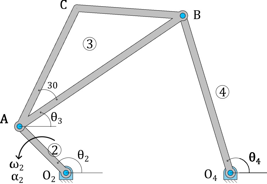
Mechanism data#
Link lengths, in meters:
\(\overline{O_2A} = 0.2\)
\(\overline{AB} = 0.6\)
\(\overline{O_4B} = 0.5\)
\(\overline{O_2O_4} = 0.5\)
\(\overline{AC} = 0.4\)
Position analysis: graphical method#
The objective is to construct the mechanism’s configuration to scale for the instant \(\theta_2 = 135^\circ\) and measure the requested coordinates and angles.
Construction Data:#
Link 1 (Frame): \(L_1 = \overline{O_2O_4} = 0.5 \text{ m}\)
Link 2 (Crank): \(L_2 = \overline{O_2A} = 0.2 \text{ m}\)
Link 3 (Coupler): \(L_3 = \overline{AB} = 0.6 \text{ m}\)
Link 4 (Rocker): \(L_4 = \overline{O_4B} = 0.5 \text{ m}\)
Point of Interest C: Located on the coupler, with \(\overline{AC} = 0.4 \text{ m}\) and a fixed angle of \(30^\circ\) counter-clockwise with respect to the segment AB.
Construction Procedure:#
Establish the frame (Link 1)
A global coordinate system is defined. The fixed pivot \(O_2\) is located at the origin (0,0).
The second fixed pivot \(O_4\) is located at (0.5, 0), establishing the length and position of the fixed link.
Position the crank (Link 2)
From \(O_2\), link 2 is drawn with its length \(L_2 = 0.2 \text{ m}\) and the input angle \(\theta_2 = 135^\circ\). The end of this vector is the position of joint A.
The coordinates of A can be calculated directly for verification: \(A = (L_2 \cos\theta_2, L_2 \sin\theta_2)\).
Locate joint B (Loop closure)
Coupler Constraint: Point B must be at a distance \(L_3 = 0.6 \text{ m}\) from A. Geometrically, this is a circle with center A and radius 0.6.
Rocker Constraint: Point B must also be at a distance \(L_4 = 0.5 \text{ m}\) from \(O_4\). Geometrically, this is a circle with center \(O_4\) and radius 0.5.
Resolve configuration ambiguity
The intersection of the two circles from the previous step gives two possible solutions for point B. These two solutions define the two configurations (or branches) of the mechanism:
Open Configuration: Generally the one with the larger angle \(\angle O_4BA\) (the “elbow” outwards).
Crossed Configuration: The one with the smaller angle \(\angle O_4BA\) (the “elbow” inwards).
The upper solution for B is chosen, corresponding to the open configuration.
Locate the point of interest C
Point C forms a rigid triangle ABC with the coupler link.
The segment AB is drawn, which defines the orientation of the coupler.
The vector \(\vec{AC}\) is constructed with a magnitude of 0.4 m, rotated \(30^\circ\) counter-clockwise with respect to the direction of the vector \(\vec{AB}\). The end of this vector is point C.
Measurement of results
With the mechanism completely drawn, the desired quantities are measured directly from the graphical software:
Coordinates of point C: \((x_C, y_C)\).
Angle of the coupler, \(\theta_3\): The angle of the segment AB with the horizontal.
Angle of the rocker, \(\theta_4\): The angle of the segment \(O_4B\) with the horizontal.
The following GeoGebra model shows the result of carrying out this process:
Position analysis: analytical method#
The objective is to find expressions for the unknowns (\(\theta_3\), \(\theta_4\), and the coordinates of C) as a function of the known parameters.
Vector Loop Formulation#
We model the mechanism as a closed chain of position vectors. Starting from \(O_2\) and returning to \(O_2\), the sum of the vectors must be zero. \( \vec{L}_2 + \vec{L}_3 - \vec{L}_4 - \vec{L}_1 = 0 \) We rearrange the equation to isolate the vectors with the unknowns: \( \vec{L}_2 + \vec{L}_3 = \vec{L}_1 + \vec{L}_4 \) Now, we decompose this vector equation into its scalar components (x and y):
x-component (real): \( L_2\cos\theta_2 + L_3\cos\theta_3 = L_1 + L_4\cos\theta_4 \quad (\text{Equation 1}) \)
y-component (imaginary): \( L_2\sin\theta_2 + L_3\sin\theta_3 = L_4\sin\theta_4 \quad (\text{Equation 2}) \)
We have a system of two nonlinear equations with two unknowns, \(\theta_3\) and \(\theta_4\).
Solving for \(\theta_3\) and \(\theta_4\)#
One way to solve the system is by using Freudenstein’s Equation, which relates the input and output angles: \( K_1\cos\theta_3 + K_2\cos\theta_2 + K_3 = \cos(\theta_2 - \theta_3) \) Where the constants \(K_1, K_2, K_3\) depend only on the link lengths:
\(K_1 = L_1 / L_2\)
\(K_2 = L_1 / L_4\)
\(K_3 = (L_2^2 - L_3^2 + L_4^2 + L_1^2) / (2L_2L_4)\)
Solving the system for \(\theta_3\) and \(\theta_4\) yields an equation of the form \(A\cos\theta_3 + B\sin\theta_3 = C\), which has standard solutions. The final solutions are: \( \theta_4 = 2 \arctan\left(\frac{-B \pm \sqrt{B^2 - 4AC}}{2A}\right) \) \( \theta_3 = \arctan\left(\frac{L_4\sin\theta_4 - L_2\sin\theta_2}{L_1 + L_4\cos\theta_4 - L_2\cos\theta_2}\right) \) Where:
\(A = \cos\theta_2 - K_1 - K_2\cos\theta_2 + K_3\)
\(B = -2\sin\theta_2\)
\(C = K_1 - (K_2+1)\cos\theta_2 + K_3\)
The \(\pm\) sign in the square root gives us the two solutions corresponding to the open and crossed configurations.
Calculation of the Coordinates of Point C#
Once \(\theta_3\) and \(\theta_4\) are calculated:
Coordinates of A:
\(x_A = L_2\cos\theta_2\)
\(y_A = L_2\sin\theta_2\)
Coordinates of C: Point C is on link 3. Its position is defined by the vector \(\vec{R}_C = \vec{R}_A + \vec{R}_{AC}\). The vector \(\vec{R}_{AC}\) has a constant magnitude of 0.4 m and an angle that is the angle of link 3 (\(\theta_3\)) plus the fixed angle of \(30^\circ\) (\(\delta_3\)).
\(x_C = x_A + \overline{AC}\cos(\theta_3 + \delta_3)\)
\(y_C = y_A + \overline{AC}\sin(\theta_3 + \delta_3)\)
Numerical Calculation for the Example#
Next, the detailed numerical calculation is performed. It is crucial to clarify that the system has two mathematical solutions, which correspond to two different physical assemblies of the mechanism.
1. The Two Possible Configurations:
By solving the vector loop equations, two valid solutions are found:
Solution 1: Open Configuration
This is the configuration shown in the figure, where the polygon \(O_2ABO_4\) is convex and the links do not cross.
The angles are: \(\mathbf{\theta_3 \approx 34.18^\circ}\) and \(\mathbf{\theta_4 \approx 106.86^\circ}\).
This is the correct solution that matches GeoGebra.
Solution 2: Crossed Configuration
In this configuration, the coupler link (AB) would cross the frame (\(O_2O_4\)).
The angles are: \(\theta_3 \approx -59.04^\circ\) and \(\theta_4 \approx 228.21^\circ\).
This solution, although mathematically valid, does not correspond to the problem figure.
2. Calculation of Coordinates for the Open Configuration:
We use the angles from the correct configuration (the open one) for the calculations.
Initial Data:
Lengths: \(L_1=0.5, L_2=0.2, L_3=0.6, L_4=0.5, \overline{AC}=0.4\)
Angles: \(\theta_2 = 135^\circ\), \(\delta_3 = 30^\circ\)
Coordinates of A:
\(x_A = L_2\cos\theta_2 = 0.2 \cos(135^\circ) = -0.1414 \text{ m}\)
\(y_A = L_2\sin\theta_2 = 0.2 \sin(135^\circ) = 0.1414 \text{ m}\)
\(A = (-0.1414, 0.1414)\)
Coordinates of C: The absolute angle of the vector \(\vec{AC}\) is \(\theta_3 + \delta_3 = 34.18^\circ + 30^\circ = 64.18^\circ\).
\(x_C = x_A + \overline{AC}\cos(\theta_3 + \delta_3) = -0.1414 + 0.4\cos(64.18^\circ) = -0.1414 + 0.1742 = 0.0328 \text{ m}\)
\(y_C = y_A + \overline{AC}\sin(\theta_3 + \delta_3) = 0.1414 + 0.4\sin(64.18^\circ) = 0.1414 + 0.3601 = 0.5015 \text{ m}\)
\(C = (0.0328, 0.5015)\)
3. Final Verified Results:
\(\theta_3 = 34.18^\circ\)
\(\theta_4 = 106.86^\circ\)
Coordinates of C: (0.0328, 0.5015) m
Velocity analysis#
At the instant when \(\theta_2 = 135^{\circ}\), the angular velocity of the input link is \(\vec{\omega}_2 = 2\hat{k}\) rad/s. Calculate the velocity of point C and the angular velocity of link 4.
Data from the position analysis: \(\theta_3 = 34.18^{\circ};\, \theta_4 = 106.86^{\circ}\) \(\vec{r}_{O2A} = -0.141\hat{i} + 0.141\hat{j}\) \(\vec{r}_{AB} = 0.496\hat{i} + 0.337\hat{j}\) \(\vec{r}_{O4B} = -0.145\hat{i} + 0.478\hat{j}\) \(\vec{r}_{AC} = 0.174\hat{i} + 0.360\hat{j}\)
Resolution#
We start by finding the velocity of point A: \(\vec{v}_A = \vec{\omega}_2 \times \vec{r}_{O2A} = 2\hat{k} \times (-0.141\hat{i} + 0.141\hat{j}) = -0.282\hat{i} - 0.282\hat{j}\) m/s.
Now we write the relative velocity equation for point B: \(\vec{v}_B = \vec{v}_A + \vec{v}_{B/A} = \vec{v}_A + \vec{\omega}_3 \times \vec{r}_{AB}\) \(\vec{v}_B = -0.282\hat{i} - 0.282\hat{j} + \omega_3\hat{k} \times (0.496\hat{i} + 0.337\hat{j})\) \(\vec{v}_B = -0.282\hat{i} - 0.282\hat{j} - 0.337\omega_3\hat{i} + 0.496\omega_3\hat{j}\) \(\vec{v}_B = (-0.282 - 0.337\omega_3)\hat{i} + (-0.282 + 0.496\omega_3)\hat{j}\)
We also express \(\vec{v}_B\) from link 4: \(\vec{v}_B = \vec{\omega}_4 \times \vec{r}_{O4B} = \omega_4\hat{k} \times (-0.145\hat{i} + 0.478\hat{j})\) \(\vec{v}_B = -0.478\omega_4\hat{i} - 0.145\omega_4\hat{j}\)
Equating the two expressions for \(\vec{v}_B\): \(-0.282 - 0.337\omega_3 = -0.478\omega_4\) \(-0.282 + 0.496\omega_3 = -0.145\omega_4\)
Solving the system of two equations for \(\omega_3\) and \(\omega_4\): \(0.478\omega_4 - 0.337\omega_3 = 0.282\) \(0.145\omega_4 + 0.496\omega_3 = 0.282\)
This yields: \(\omega_3 = 0.328\) rad/s \(\omega_4 = 0.821\) rad/s
So, \(\vec{\omega}_3 = 0.328\hat{k}\) rad/s and \(\vec{\omega}_4 = 0.821\hat{k}\) rad/s.
Finally, we calculate the velocity of point C: \(\vec{v}_C = \vec{v}_A + \vec{v}_{C/A} = \vec{v}_A + \vec{\omega}_3 \times \vec{r}_{AC}\) \(\vec{v}_C = -0.282\hat{i} - 0.282\hat{j} + 0.328\hat{k} \times (0.174\hat{i} + 0.360\hat{j})\) \(\vec{v}_C = -0.282\hat{i} - 0.282\hat{j} - 0.118\hat{i} + 0.057\hat{j}\) \(\vec{v}_C = -0.400\hat{i} - 0.225\hat{j}\) m/s.
Velocity Kinematics (Cinema)#
The following GeoGebra model shows the velocity cinema of the mechanism.
Note that to calculate the velocity of point C, one can use the concept of homology between the velocity cinema and the mechanism (a rotation of \(90^\circ\) and scaling). This way, it’s possible to find point \(c\) in the velocity cinema, which defines the end of a vector originating from \(O_v\) that determines the velocity of C, \(\vec{v}_C\). This point is found at a distance \(\overline{ac}=\frac{\overline{ab}}{\overline{AB}}\overline{AC}\) on the segment \(ab\), and is then rotated 30 degrees counter-clockwise, as was done to obtain point C in the mechanism’s construction.
Acceleration analysis#
At the instant when the crank forms an angle \(\theta_2 = 135^{\circ}\) with the horizontal, its angular velocity is \(\vec{\omega}_2 = 2\hat{k}\) rad/s, and its acceleration is \(\vec{\alpha}_2 = -1.5\hat{k}\) rad/s². Calculate the acceleration of point C and the angular acceleration of link 4.
Data:
Link lengths, in meters: \(\overline{O_2 A} = 0.2;\, \overline{AB} = 0.6;\, \overline{O_4 B} = 0.5;\, \overline{O_2 O_4} = 0.5;\, \overline{AC} = 0.4\). Angles of links 3 and 4 with the horizontal (from position analysis): \(\theta_3 = 34.18^{\circ};\, \theta_4 = 106.86^{\circ}\). And their velocities (from velocity analysis): \(\vec{\omega}_3 = 0.328\hat{k}\) rad/s; \(\vec{\omega}_4 = 0.821\hat{k}\) rad/s.
Resolution#
The procedure for calculating the mechanism’s accelerations is similar to that for velocities. We start with point A as we have information about it. We calculate \(\vec{a}_A\) from its normal and tangential components:
\(\vec{a}_A = \vec{a}_A^n + \vec{a}_A^t = \vec{\omega}_2 \times (\vec{\omega}_2 \times \vec{r}_{O2A}) + \vec{\alpha}_2 \times \vec{r}_{O2A}\) \(\vec{a}_A = 2\hat{k} \times (2\hat{k} \times (-0.141\hat{i} + 0.141\hat{j})) - 1.5\hat{k} \times (-0.141\hat{i} + 0.141\hat{j}) = 0.777\hat{i} - 0.353\hat{j}\)
Now, analyzing point B as part of link 3, we have:
\(\vec{a}_B = \vec{a}_A + \vec{a}_{B/A}\)
which, by decomposing, gives:
\(\vec{a}_B^n + \vec{a}_B^t = \vec{a}_A + \vec{a}_{B/A}^n + \vec{a}_{B/A}^t\)
where the acceleration of A is known, and we can express the components of the relative acceleration from the available information:
For \(\vec{a}_{B/A}^n\), everything is known. Therefore: \(\vec{a}_{B/A}^n = \vec{\omega}_3 \times (\vec{\omega}_3 \times \vec{r}_{AB}) = -0.053\hat{i} - 0.036\hat{j}\)
For \(\vec{a}_{B/A}^t\), we can operate and express it in terms of the unknown \(\vec{\alpha}_3\), of which we only know its direction: \(\vec{a}_{B/A}^t = \vec{\alpha}_3 \times \vec{r}_{AB} = \alpha_3\hat{k} \times (0.496\hat{i} + 0.337\hat{j}) = -0.337\alpha_3\hat{i} + 0.496\alpha_3\hat{j}\)
On the other hand, if we consider point B as part of link 4, we have:
For \(\vec{a}_B^n\), of which we know everything: \(\vec{a}_B^n = \vec{\omega}_4 \times (\vec{\omega}_4 \times \vec{r}_{O4B}) = 0.098\hat{i} - 0.324\hat{j}\)
For \(\vec{a}_B^t\), of which we don’t know \(\vec{\alpha}_4\): \(\vec{a}_B^t = \vec{\alpha}_4 \times \vec{r}_{O4B} = \alpha_4\hat{k} \times (-0.145\hat{i} + 0.478\hat{j}) = -0.478\alpha_4\hat{i} - 0.145\alpha_4\hat{j}\)
Finally, if we equate both expressions, we have:
\(0.098\hat{i} - 0.324\hat{j} - 0.478\alpha_4\hat{i} - 0.145\alpha_4\hat{j} = 0.777\hat{i} - 0.353\hat{j} - 0.053\hat{i} - 0.036\hat{j} - 0.337\alpha_3\hat{i} + 0.496\alpha_3\hat{j}\)
From which it is possible to obtain a system of two equations with two unknowns, \(\alpha_3\) and \(\alpha_4\), once we decompose into \(\hat{i}\) and \(\hat{j}\):
\(0.098 - 0.478\alpha_4 = 0.777 - 0.053 - 0.337\alpha_3\) \(-0.324 - 0.145\alpha_4 = -0.353 - 0.036 + 0.496\alpha_3\)
whose solution gives us:
\(\alpha_3 = 0.427\) \(\alpha_4 = -1.007\)
which, knowing the direction, we can express in vector form:
\(\vec{\alpha}_3 = 0.427\hat{k}\) rad/s²; \(\vec{\alpha}_4 = -1.007\hat{k}\) rad/s²
Finally, to calculate the acceleration of point C, we apply relative accelerations between C and A:
\(\vec{a}_C = \vec{a}_A + \vec{a}_{C/A}^n + \vec{a}_{C/A}^t = 0.777\hat{i} - 0.353\hat{j} + \vec{\omega}_3 \times (\vec{\omega}_3 \times \vec{r}_{AC}) + \vec{\alpha}_3 \times \vec{r}_{AC}\) \(\vec{a}_C = 0.777\hat{i} - 0.353\hat{j} + 0.328\hat{k} \times (0.328\hat{k} \times (0.174\hat{i} + 0.360\hat{j})) + 0.427\hat{k} \times (0.174\hat{i} + 0.360\hat{j}) = 0.605\hat{i} - 0.318\hat{j}\) m/s²
Acceleration Cinema#
The following GeoGebra model shows the acceleration cinema of the mechanism.
Note that to calculate the acceleration of point C, one can use the concept of homology between the acceleration cinema and the mechanism (a rotation of \(180^\circ\) and scaling). This way, it’s possible to find point \(c'\) in the acceleration cinema, which defines the end of a vector originating from \(O_a\) that determines the acceleration of C, \(\vec{a}_C\). This point is found at a distance \(\overline{a'c'}=\frac{\overline{a'b'}}{\overline{AB}}\overline{AC}\) on the segment \(a'b'\), and is then rotated 30 degrees counter-clockwise, as was done to obtain point C in the mechanism’s construction.