Rigid body dynamics

Moving from particles to bodies with extension brings new quantities: orientation, angular velocity and angular acceleration. We need to extend the equations of the particle to solids with an area or a volume:

• Linear motion (\(\vec{p}\)) \(\rightarrow\) Newton’s equations.

• Angular motion (\(\vec{L}\)) \(\rightarrow\) Euler’s equations.

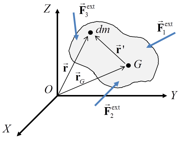
Consider a body divided into infinitesimal mass elements \(dm\), with center of mass (or of gravity) \(G\), under a set of external point forces \(\vec{F}_j^{ext}\). Let \(\vec{r}\) be the position of each \(dm\) from the origin \(O\) and \(\vec{r}\,'\) its position relative to \(G\).

Newton’s equation

Applying Newton’s second law to each element \(dm\) and adding up (integrating) over the whole body, we get the external forces and the internal forces \(d\vec{F}^i\) between the elements:

\[ \int_V d\vec{F}^i + \sum_j \vec{F}_j^{ext} = \int_V \vec{a}\, dm \]

By Newton’s third law (action and reaction), internal forces cancel out in pairs, and their integral is zero. Calling \(\vec{F}^{ext}\) the resultant of the external forces:

\[ \vec{F}^{ext} = \int_V \vec{a}\, dm = \int_V \frac{d^2\vec{r}}{dt^2}\, dm = \frac{d^2}{dt^2} \underbrace{\int_V \vec{r}\, dm}_{m\,\vec{r}_G} = m \ddot{\vec{r}}_G \]

where we used the definition of the center of mass, \(\vec{r}_G = \frac{1}{m}\int_V \vec{r}\,dm\).

Newton’s equation of a rigid body

\[ \sum_j \vec{F}_j^{ext} = m\, \vec{a}_G \]

These are 2 scalar equations in the plane and 3 in space. As far as translation is concerned, the body behaves as a particle with all its mass concentrated at \(G\).

Euler’s equation

We now take moments about the center of mass \(G\), using the vectors \(\vec{r}\,'\):

\[ \int_V \vec{r}\,' \times d\vec{F}^i + \sum_j \vec{r}_j\,' \times \vec{F}_j^{ext} = \int_V \vec{r}\,' \times \vec{a}\, dm \]

Again, the moments of the internal forces cancel out in pairs. Calling \(\vec{M}^{ext}_G\) the resultant moment of the external forces (and torques) about \(G\):

\[ \vec{M}^{ext}_G = \int_V \vec{r}\,' \times \vec{a}\, dm \]

This integral is more involved than the one in Newton’s equation. Using the velocity field of a rigid body relative to \(G\), \(\vec{v} = \vec{v}_G + \vec{\omega} \times \vec{r}\,'\), and the rules for differentiating vectors, we arrive at:

\[ \sum_j \vec{M}_j^{ext} = \frac{d}{dt} \left[ \underbrace{ \int_V \left\{ |\vec{r}\,'|^2\, \mathbf{I}_3 - \vec{r}\,'\vec{r}\,'^\top \right\} dm }_{\mathbf{I}_G} \vec{\omega} \right] \]

where a new concept appears: the inertia tensor (or matrix) \(\mathbf{I}_G\) about \(G\), which measures the resistance of the body to changes in its rotation. The term in brackets is the angular momentum of the body about \(G\), \(\vec{L}_G = \mathbf{I}_G \vec{\omega}\).

Inertia tensor

With \(\vec{r}\,' = (x', y', z')\):

\[\begin{split} \begin{aligned} \mathbf{I}_G &= \int_V |\vec{r}\,'|^2 \mathbf{I}_3 - \vec{r}\,'\vec{r}\,'^\top dm = \int_V \left( x'^2+y'^2+z'^2 \right) \begin{bmatrix} 1 & 0 & 0 \\ 0 & 1 & 0 \\ 0 & 0 & 1 \end{bmatrix} - \begin{bmatrix} x' \\ y' \\ z' \end{bmatrix} \begin{bmatrix} x' & y' & z' \end{bmatrix} dm \\ &= \int_V \begin{bmatrix} y'^2+z'^2 & -x'y' & -x'z' \\ -x'y' & x'^2+z'^2 & -y'z' \\ -x'z' & -y'z' & x'^2+y'^2 \end{bmatrix} dm = \begin{bmatrix} I_x & -I_{xy} & -I_{xz} \\ -I_{yx} & I_y & -I_{yz} \\ -I_{zx} & -I_{zy} & I_z \end{bmatrix} \end{aligned} \end{split}\]

The diagonal terms are the moments of inertia and the off-diagonal ones, the products of inertia. They depend on the shape of the body and on its mass distribution: they are computed or taken from tables (see Computing inertias in 2D).

Euler’s equation in 3D

Differentiating the product:

\[ \sum_j \vec{M}_j^{ext} = \frac{d}{dt}\left( \mathbf{I}_G \vec{\omega} \right) = \mathbf{I}_G \dot{\vec{\omega}} + \dot{\mathbf{I}}_G \vec{\omega} \]

\(\mathbf{I}_G\) is constant when expressed in body-fixed axes; when expressed in fixed axes, its derivative gives rise to a gyroscopic term, and we get:

Euler’s equations of a rigid body (3D)

\[ \underbrace{\sum_j \vec{M}_j^{ext}}_{3\times 1} = \underbrace{\mathbf{I}_G}_{3\times 3}\, \underbrace{\vec{\alpha}}_{3\times 1} + \underbrace{\vec{\omega}}_{3\times 1} \times \underbrace{\mathbf{I}_G \vec{\omega}}_{3\times 1} \]

They relate the applied moments to the change of angular velocity.

Euler’s equation in the plane (2D)

In a planar mechanism, \(\vec{\omega} = \omega\,\hat{k}\) and \(\vec{\alpha} = \alpha\,\hat{k}\), and if the plane of motion is a plane of symmetry of the link, \(I_{xz} = I_{yz} = 0\):

\[\begin{split} \begin{bmatrix} 0 \\ 0 \\ M^{ext}_z \end{bmatrix} = \begin{bmatrix} I_x & -I_{xy} & 0 \\ -I_{yx} & I_y & 0 \\ 0 & 0 & I_z \end{bmatrix}_G \begin{bmatrix} 0 \\ 0 \\ \alpha \end{bmatrix} + \underbrace{\begin{bmatrix} 0 \\ 0 \\ \omega \end{bmatrix} \times \begin{bmatrix} 0 \\ 0 \\ I_z \omega \end{bmatrix}}_{=\vec{0}} = \begin{bmatrix} 0 \\ 0 \\ I_{z,G}\, \alpha \end{bmatrix} \end{split}\]

A single scalar equation is left:

Euler’s equation of a planar body

\[ \sum_j M^{ext}_{j,z} = I_{z,G}\, \alpha \]

with \(I_{z,G}\) the only relevant moment of inertia:

\[ I_{z,G} = \int_{\text{area}} \left( x'^2 + y'^2 \right) dm \]

Newton-Euler equations

A general rigid body satisfies two sets of equations:

\[\begin{split} \begin{aligned} \sum_j \vec{F}_j^{ext} &= m\, \vec{a}_G & &\text{(Newton: position of } G\text{)} \\ \sum_j \vec{M}_{j,G}^{ext} &= \mathbf{I}_G \vec{\alpha} + \vec{\omega} \times \mathbf{I}_G \vec{\omega} & &\text{(Euler: orientation)} \end{aligned} \end{split}\]

\(\vec{a}_G = \ddot{\vec{r}}_G\) describes how the position of the center of mass evolves. To integrate the orientation, we must choose how to parameterize it, for instance with Euler angles \(\vec{\psi} = (\psi_1, \psi_2, \psi_3)\) (yaw, pitch and roll). The angular velocity is not the derivative of those angles, but a linear combination of them, \(\vec{\omega} = \mathbf{B}(\vec{\psi})\,\dot{\vec{\psi}}\), with:

\[\begin{split} \mathbf{B} = \begin{bmatrix} 0 & -\sin\psi_1 & \cos\psi_1\cos\psi_2 \\ 0 & \cos\psi_1 & \sin\psi_1\cos\psi_2 \\ 1 & 0 & -\sin\psi_2 \end{bmatrix}, \qquad \dot{\vec{\omega}} = \mathbf{B}\ddot{\vec{\psi}} + \dot{\mathbf{B}}\dot{\vec{\psi}} \end{split}\]

Substituting, we arrive at a system of ordinary differential equations that can be integrated numerically, which allows simulating any system of free rigid bodies in 3D given the forces and the inertias:

\[\begin{split} \begin{aligned} \sum_j \vec{F}_j^{ext} &= m \ddot{\vec{r}}_G \\ \sum_j \vec{M}_j^{ext} &= \mathbf{I}_G \mathbf{B} \ddot{\vec{\psi}} + \mathbf{I}_G \dot{\mathbf{B}} \dot{\vec{\psi}} + (\mathbf{B}\dot{\vec{\psi}}) \times \mathbf{I}_G (\mathbf{B}\dot{\vec{\psi}}) \end{aligned} \qquad\rightarrow\qquad \left\{ \begin{aligned} \ddot{\vec{r}}_G &= \vec{f}_N(\vec{r}_G, \dot{\vec{r}}_G, \vec{\psi}, \dot{\vec{\psi}}) \\ \ddot{\vec{\psi}} &= \vec{f}_E(\vec{r}_G, \dot{\vec{r}}_G, \vec{\psi}, \dot{\vec{\psi}}) \end{aligned} \right. \end{split}\]

In the planar case, calling \(\theta(t)\) the orientation of the link (rotation about \(z\)), the terms with \(\dot{\mathbf{B}}\) and the cross product vanish, leaving three scalar equations per link:

Newton-Euler equations in the plane

\[\begin{split} \left\{ \begin{aligned} \sum_j F^{ext}_{j,x} &= m\, a_{G,x} \\ \sum_j F^{ext}_{j,y} &= m\, a_{G,y} \\ \sum_j M^{ext}_{j,z} &= I_{z,G}\, \ddot{\theta} = I_{z,G}\, \alpha \end{aligned} \right. \end{split}\]

Watch out! The moment equation is written about the center of mass \(G\). If moments are taken about another point \(P\), the moment of \(m\vec{a}_G\) about \(P\) must be added (or, equivalently, D’Alembert’s principle must be used, see D’Alembert’s principle).

Example: bodies rolling down a ramp. Four bodies with the same mass and radius roll without slipping down a ramp. Their moments of inertia, relative to \(k = mR^2\), are (back to front): \(0.66\,k\) (hollow sphere), \(0.4\,k\) (solid sphere), \(1.0\,k\) (hollow cylinder) and \(0.5\,k\) (solid cylinder). The smaller the inertia, the larger the acceleration, and the sooner the body reaches the bottom.

(Credits: Lucas V. Barbosa, public domain.)

Angular momentum, stability and balancing

If the resultant moment of the external forces is zero, the angular momentum of the body is conserved:

\[ \vec{M}_G = \dot{\vec{L}}_G = \vec{0} \quad\rightarrow\quad \vec{L}_G = \mathbf{I}_G \vec{\omega} = \text{constant} \]

Careful! This does not mean that the angular velocity \(\vec{\omega}\) is constant: in general, the direction of \(\vec{L}_G\) does not coincide with that of \(\vec{\omega}\). The so-called “tennis racket theorem” (or Dzhanibekov effect) is a very visual case: rotation about the intermediate axis of inertia is unstable, and the body flips periodically while keeping its angular momentum.

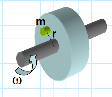
This same gyroscopic term causes trouble in shafts, rotors and wheels whose rotation axis does not coincide with a principal axis of the inertia tensor: moments appear that produce vibrations and damage the bearings. This is studied in the balancing lesson (lesson 5).