Example 2.15: Bicycle suspension (graphical method)

The mechanism in the photo (dimensions in centimeters) shows the rear suspension of a bicycle (January 2023 exam). It is the same mechanism solved analytically in Example 2.9: Bicycle suspension. Find:

1. All the absolute instantaneous centers of rotation (ICRs).

2. The velocity of point \(A\), by the graphical method.

3. From the acceleration polygon given below, the angular accelerations of all the bodies.

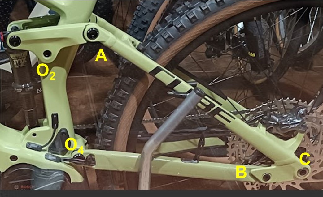
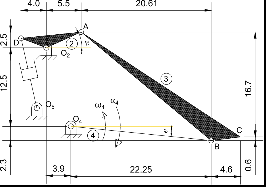
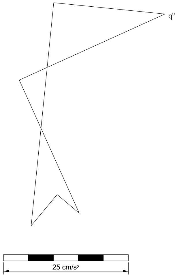
Data: \(\omega_4 = 1\) rad/s counterclockwise, \(\alpha_4 = 2\) rad/s² clockwise. Any other dimension can be measured with the scale bars.

Solution

1. Absolute ICRs

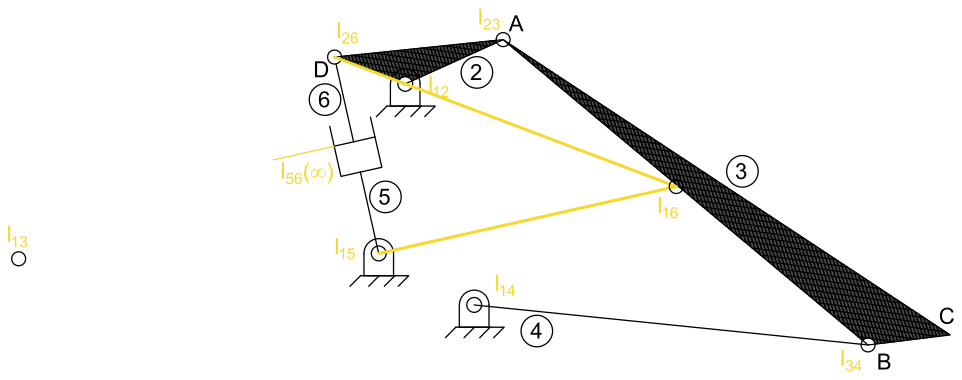
The mechanism has \(N = 6\) bodies: 1 frame (ground), 2 rocker \(DO_2A\), 3 swingarm \(ABC\), 4 link \(O_4B\), 5 shock cylinder and 6 shock rod. So there are \(6 \cdot 5 / 2 = 15\) ICRs, of which the absolute ones are required: \(I_{12}\), \(I_{13}\), \(I_{14}\), \(I_{15}\) and \(I_{16}\).

First, all the ICRs that can be seen directly: the pin joints between pairs of bodies in contact (\(I_{12}\), \(I_{23}\), \(I_{34}\), \(I_{14}\), \(I_{15}\) and \(I_{26}\)), and \(I_{56}\), which is at infinity in the direction perpendicular to the shock axis, since the rod slides inside the cylinder. Of the absolute ICRs, only \(I_{13}\) and \(I_{16}\) are still unknown.

To find \(I_{13}\), apply Kennedy’s theorem twice (see Example 2.14: Instantaneous centers of a four-bar linkage for a detailed explanation), with the pairs \(I_{12}\)-\(I_{23}\) and \(I_{14}\)-\(I_{34}\). Each pair defines a line, and the ICR is at their intersection:

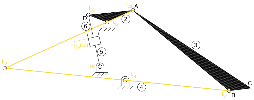
Finally, \(I_{16}\) is found with the pairs \(I_{15}\)-\(I_{56}\) (the line through \(O_5\) perpendicular to the shock axis) and \(I_{12}\)-\(I_{26}\):

2. Velocity of A

Even with the graphical method, we must first write the equations that determine the velocities, following a loop that goes through all the bodies of the kinematic chain to analyze. Here, the loop is \(O_4\)-\(B\)-\(A\)-\(O_2\), which gives the following relative velocity equations:

\[\begin{split} \begin{aligned} \vec{v}_B &= \cancel{\vec{v}_{O_4}} + \omega_4\,\hat{k} \times \vec{r}_{O_4B} && \text{(Body 4)} \\ \vec{v}_A &= \vec{v}_B + \omega_3\,\hat{k} \times \vec{r}_{BA} && \text{(Body 3)} \\ \vec{v}_A &= \cancel{\vec{v}_{O_2}} + \omega_2\,\hat{k} \times \vec{r}_{O_2A} && \text{(Body 2)} \end{aligned} \end{split}\]

For the graphical method it is convenient to combine them into a single vector equation: substitute \(\vec{v}_B\) from the first equation into the second, and equate the right-hand sides of the second and third, since both are \(\vec{v}_A\):

\[ \underbrace{\omega_2\,\hat{k} \times \vec{r}_{O_2A}}_{\perp\, O_2A} = \underbrace{\omega_4\,\hat{k} \times \vec{r}_{O_4B}}_{\text{known}} + \underbrace{\omega_3\,\hat{k} \times \vec{r}_{BA}}_{\perp\, AB} \]

where we have marked which term is fully known (magnitude and direction), and which are known only in direction (perpendicular to their links) but not in magnitude. From the data, \(|\omega_4|\,\overline{O_4B} = 1~\text{rad/s} \cdot \sqrt{22.25^2 + 2.3^2}~\text{cm} = 22.35\) cm/s. Drawing this equation to scale gives the following velocity polygon:

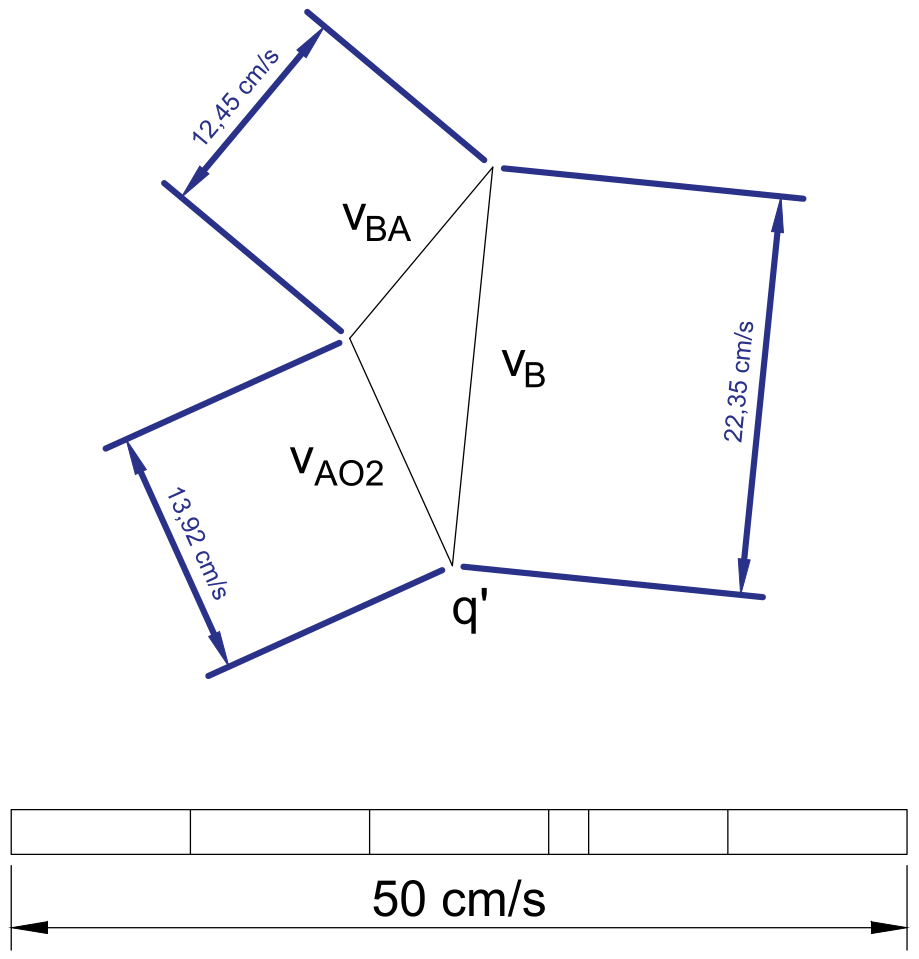
from which we measure:

• \(|\vec{v}_{AO_2}| = |\vec{v}_A| = 13.92\) cm/s, the requested value.

• \(|\vec{v}_{BA}| = 12.45\) cm/s, from which \(|\omega_3| = |\vec{v}_{BA}| / \overline{BA} = 12.45 / 26.91 = 0.46\) rad/s, counterclockwise.

3. Angular accelerations

As for the velocities, it is convenient to write the equations explicitly, to identify each vector of the polygon:

\[\begin{split} \begin{aligned} \vec{a}_B &= \cancel{\vec{a}_{O_4}} + \alpha_4\,\hat{k} \times \vec{r}_{O_4B} - \omega_4^2\,\vec{r}_{O_4B} && \text{(Body 4)} \\ \vec{a}_A &= \vec{a}_B + \alpha_3\,\hat{k} \times \vec{r}_{BA} - \omega_3^2\,\vec{r}_{BA} && \text{(Body 3)} \\ \vec{a}_A &= \cancel{\vec{a}_{O_2}} + \alpha_2\,\hat{k} \times \vec{r}_{O_2A} - \omega_2^2\,\vec{r}_{O_2A} && \text{(Body 2)} \end{aligned} \end{split}\]

which, combined into a single equation:

\[ \underbrace{\alpha_2\,\hat{k} \times \vec{r}_{O_2A}}_{\vec{a}^t_A} \underbrace{- \,\omega_2^2\,\vec{r}_{O_2A}}_{\vec{a}^n_A} = \underbrace{\alpha_4\,\hat{k} \times \vec{r}_{O_4B}}_{\vec{a}^t_B} \underbrace{- \,\omega_4^2\,\vec{r}_{O_4B}}_{\vec{a}^n_B} + \underbrace{\alpha_3\,\hat{k} \times \vec{r}_{BA}}_{\vec{a}^t_{BA}} \underbrace{- \,\omega_3^2\,\vec{r}_{BA}}_{\vec{a}^n_{BA}} \]

allows identifying each vector of the given polygon by its direction (parallel or perpendicular to each link). The normal components are known from the angular velocities, and \(\vec{a}^t_B\) from the given \(\alpha_4\); the step-by-step construction below shows how the polygon is built. Measuring on the polygon:

• \(|\vec{a}^t_{BA}| \approx 8.1\) cm/s², so \(|\alpha_3| = |\vec{a}^t_{BA}| / \overline{BA} \approx 8.1 / 26.91 \approx 0.3\) rad/s², clockwise.

• \(|\vec{a}^t_A| \approx 29.15\) cm/s², so \(|\alpha_2| = |\vec{a}^t_A| / \overline{O_2A} \approx 29.15 / 6.04 \approx 4.82\) rad/s², clockwise.

These values agree with the analytical solution of Example 2.9: Bicycle suspension: \(\alpha_3 = -0.3016\) rad/s² and \(\alpha_2 = -4.803\) rad/s².

Step-by-step constructions

Absolute ICRs, and a check of \(\vec{v}_A\) using \(I_{13}\):

Velocity polygon (part 2):

Acceleration polygon (part 3):